tf.nn.conv2,cross_entropy,loss,sklearn.preprocessing,next_batch,truncated_normal,seed,shuffle,argmax

本文主要是介绍tf.nn.conv2,cross_entropy,loss,sklearn.preprocessing,next_batch,truncated_normal,seed,shuffle,argmax，希望对大家解决编程问题提供一定的参考价值，需要的开发者们随着小编来一起学习吧！

tf.truncated_normal

https://www.tensorflow.org/api_docs/python/tf/random/truncated_normal
truncated_normal(
shape,
mean=0.0,
stddev=1.0,
dtype=tf.float32,
seed=None,
name=None
)

seed: 随机种子，若 seed 赋值，每次产生相同随机数

import tensorflow as tf
import matplotlib.pyplot as plt
tn = tf.truncated_normal([20],mean=5,stddev=1)
#sess = tf.Session()
with tf.Session() as sess:
ov = sess.run(tn)
print(ov)
plt.plot(ov)
plt.show()

卷积tf.nn.conv2d

参数：
input : 输入的要做卷积的图片，要求为一个张量，shape为 [ batch, in_height, in_weight, in_channel ]，其中batch为图片的数量，in_height 为图片高度，in_weight 为图片宽度，in_channel 为图片的通道数，灰度图该值为1，彩色图为3。（也可以用其它值，但是具体含义不是很理解）
filter： 卷积核，要求也是一个张量，shape为 [ filter_height, filter_weight, in_channel, out_channels ]，其中 filter_height 为卷积核高度，filter_weight 为卷积核宽度，in_channel 是图像通道数 ，和 input 的 in_channel 要保持一致，out_channel 是卷积核数量。
strides： 卷积时在图像每一维的步长，这是一个一维的向量，[ 1, strides, strides, 1]，第一位和最后一位固定必须是1
padding： string类型，值为“SAME” 和 “VALID”，表示的是卷积的形式，是否考虑边界。"SAME"是考虑边界，不足的时候用0去填充周围，"VALID"则不考虑
use_cudnn_on_gpu： bool类型，是否使用cudnn加速，默认为true

cross_entropy交叉熵

https://blog.csdn.net/mao_xiao_feng/article/details/53382790
https://zhuanlan.zhihu.com/p/149186719
tf.nn.softmax_cross_entropy_with_logits(logits, labels, name=None)
注意！！！这个函数的返回值并不是一个数，而是一个向量，如果要求交叉熵，我们要再做一步tf.reduce_sum操作,就是对向量里面所有元素求和，最后才得到，如果求loss，则要做一步tf.reduce_mean操作，对向量求均值！
tf.reduce_sum(tf.nn.softmax_cross_entropy_with_logits(logits, y_))#dont forget tf.reduce_sum()!!
假设一个动物照片的数据集中有5种动物，且每张照片中只有一只动物，每张照片的标签都是one-hot编码。

第一张照片是狗的概率为100%，是其他的动物的概率是0；第二张照片是狐狸的概率是100%，是其他动物的概率是0，其余照片同理；因此可以计算下，每张照片的熵都为0。换句话说，以one-hot编码作为标签的每张照片都有100%的确定度，不像别的描述概率的方式：狗的概率为90%，猫的概率为10%。

假设有两个机器学习模型对第一张照片分别作出了预测：Q1和Q2,而第一张照片的真实标签为[1,0,0,0,0]。

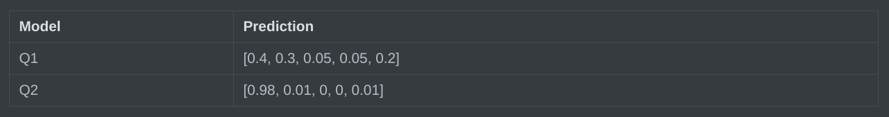
具体的执行流程大概分为两步：

第一步是先对网络最后一层的输出做一个softmax，这一步通常是求取输出属于某一类的概率，对于单样本而言，输出就是一个num_classes大小的向量（[Y1，Y2,Y3…]其中Y1，Y2，Y3…分别代表了是属于该类的概率）

softmax的公式是



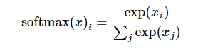
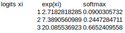
两个模型预测效果如何呢，可以分别计算下交叉熵：

交叉熵对比了模型的预测结果和数据的真实标签，随着预测越来越准确，交叉熵的值越来越小，如果预测完全正确，交叉熵的值就为0。因此，训练分类模型时，可以使用交叉熵作为损失函数。

2020年9月4日再次温习：

import tensorflow as tf#our NN's output
logits=tf.constant([[1.0,2.0,3.0],[1.0,2.0,3.0],[1.0,2.0,3.0]])
#step1:do softmax
y=tf.nn.softmax(logits)
#true label
y_=tf.constant([[0.0,0.0,1.0],[0.0,0.0,1.0],[0.0,0.0,1.0]])cross_entropy=tf.nn.softmax_cross_entropy_with_logits(logits=logits, labels=y_)#step2:do cross_entropy 
cross_entropysum = -tf.reduce_sum(y_*tf.log(y))#do cross_entropy just one step
cross_entropysum2=tf.reduce_sum(tf.nn.softmax_cross_entropy_with_logits(logits=logits, labels=y_))  #dont forget tf.reduce_sum()!!with tf.Session() as sess:softmax=sess.run(y)c_e = sess.run(cross_entropysum)c_e2 = sess.run(cross_entropysum2)cre=sess.run(cross_entropy)print("step1:softmax result=")print(softmax)print("step2:cross_entropy result=")print(cre)print("sess.run(tf.log(y)) = {sess.run(tf.log(y))}")print("step2:cross_entropy sum result=")print(c_e)print("Function(sum softmax_cross_entropy_with_logits) result=")print(c_e2)

对于一个批次， softmax为一个指数形式的概率矩阵，一个图像对应一行分类概率
交叉熵tf.nn.softmax_cross_entropy_with_logits(logits, labels, name=Non）为正确值的矢量，每个值是单幅图像的正确标号（正确分类）与softmax概率的自然对数点乘之和的和，对于单个图像，交叉熵是个标量，对于一个batch, 交叉熵是个矢量。
交叉熵求和为每个样品点乘之和的和的和，即所有样品的和
损失则再求交叉熵和的平均值。

损失函数loss

向量求均值
tf.reduce_mean(tf.nn.softmax_cross_entropy_with_logits(labels=y_, logits=y))

tf.reduce_mean axis分析示例
x = tf.constant([[1., 1.], [2., 2.]])
tf.reduce_mean(x) # 1.5
tf.reduce_mean(x, 0) # [1.5, 1.5]
tf.reduce_mean(x, 1) # [1., 2.]

精确度accuracy

correct_prediction = tf.equal(tf.argmax(y,1), tf.argmzx(y_,1))，验证模型准确率。tf.argmax从tensor寻找最大值序号，tf.argmax(y,1)求预测数字概率最大，tf.argmax(y_,1)找样本真实数字类别。tf.equal判断预测数字类别是否正确，返回计算分类操作是否正确。
accuracy = tf.reduce_mean(tf.cast(correct_prediction,tf.float32))，统计全部样本预测正确度。tf.cast转化correct_prediction输出值类型。
print(accuracy.eval({x: mnist.test.images,y_: mnist.test.labels}))。测试数据特征、Label输入评测流程，计算模型测试集准确率。Softmax Regression MNIST数据分类识别，测试集平均准确率92%左右。

    with tf.name_scope('accuracy'):correct_prediction = tf.equal(tf.argmax(logits, 1), tf.argmax(y, 1))accuracy = tf.reduce_mean(tf.cast(correct_prediction, tf.float32))# 指标变化：随着迭代进行，精度的变化情况tf.summary.scalar('accuracy', accuracy)# 把所有要显示的参数聚在一起summ = tf.summary.merge_all()sess.run(tf.global_variables_initializer())# 保存路径tenboard_dir = './tensorboard/test3/'# 指定一个文件用来保存图writer = tf.summary.FileWriter(tenboard_dir + hparam)# 把图add进去writer.add_graph(sess.graph)for i in range(2001):batch = mnist.train.next_batch(100)# 每迭代5次对结果进行保存if i % 5 == 0:[train_accuracy, s] = sess.run([accuracy, summ], feed_dict={x: batch[0], y: batch[1]})writer.add_summary(s, i)sess.run(train_step, feed_dict={x: batch[0], y: batch[1]})

tf.argmax(input, axis=None, name=None, dimension=None)
此函数是对矩阵按行或列计算最大值，输出最大值的下标
参数
input：输入Tensor
axis：0表示按列，1表示按行
name：名称
dimension：和axis功能一样，默认axis取值优先。新加的字段
返回：Tensor 一般是行或列的最大值下标向量
https://blog.csdn.net/ZHANGHUIHUIA/article/details/83784943

global_variables_initializer

所有变量需要初始化
sess.run(tf.global_variables_initializer())
或
init = tf.initialize_all_variables()
with tf.Session() as sess:
sess.run(init)

维数－1意义

https://stackoverflow.com/questions/18691084/what-does-1-mean-in-numpy-reshape
numpy allow us to give one of new shape parameter as -1 (eg: (2,-1) or (-1,3) but not (-1, -1)). It simply means that it is an unknown dimension and we want numpy to figure it out. And numpy will figure this by looking at the ‘length of the array and remaining dimensions’ and making sure it satisfies the above mentioned criteria

mnist.train.next_batch()和shuffle选项

https://blog.csdn.net/weixin_42104955/article/details/102576382
mnist.train.next_batch()内部是有shuffle=True默认值的，如果不设置为False，那么每一次训练的结果都会不一样。
对于numpy数组对其数组进行重新排序的方法：将变序数组镶入待修改数组的索引值。如下例：

suffle作用

import numpy as np
test = np.array([[1, 1, 1],[2, 2, 2],[3, 3, 3],[4, 4, 4]])
disorder = np.arange(4)
np.random.shuffle(disorder)
test=test[disorder]
print(disorder)
print("改变后数组\n",test)

结果

[3 2 0 1]
改变后数组[[4 4 4][3 3 3][1 1 1][2 2 2]]

MNIST进阶之next_batch()
https://blog.csdn.net/qq_33254870/article/details/81390897
函数原型：
def next_batch(self, batch_size, fake_data=False, shuffle=True)

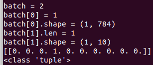
batch=mnist.train.next_batch(1)
print("batch = {}".format(len(batch)))
print("batch[0] = {}".format(len(batch[0]))) 
print("batch[0].shape = {}".format(batch[0].shape))
print("batch[1].len = %d"%len(batch[1]))
print("batch[1].shape = {}".format(batch[1].shape))

batch=mnist.train.next_batch(3)

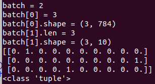
batch为元组类型, python 的元组与列表类似，不同之处在于元组的元素不能修改。
元组使用小括号，列表使用方括号。
元组创建很简单，只需要在括号中添加元素，并使用逗号隔开即可。
batch元组没有shape, 但batch[0], batch[1]有shape, 前者代表一个batchsize所有数据，后者代表所有金标labeltr

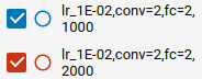
保持训练结果的一致性，必须设置next_batch()设置shuffle=False, tf.truncated_normal() 赋值seed

下图为1000与2000pcs，结果基本保持一致

mnist example 1

https://www.cnblogs.com/lizheng114/p/7439556.html
mnist = input_data.read_data_sets(FLAGS.data_dir, one_hot=True)
x是特征值
x = tf.placeholder(tf.float32, [None, 784])
w表示每一个特征值（像素点）会影响结果的权重
W = tf.Variable(tf.zeros([784, 10]))
b = tf.Variable(tf.zeros([10]))
y = tf.matmul(x, W) + b
y_ 是图片实际对应的值
y_ = tf.placeholder(tf.float32, [None, 10])

cross_entropy = tf.reduce_mean(tf.nn.softmax_cross_entropy_with_logits(labels=y_, logits=y))
train_step = tf.train.GradientDescentOptimizer(0.5).minimize(cross_entropy)
sess = tf.InteractiveSession()
tf.global_variables_initializer().run()
mnist.train 训练数据
for _ in range(1000):
batch_xs, batch_ys = mnist.train.next_batch(100)
sess.run(train_step, feed_dict={x: batch_xs, y_: batch_ys})

#取得y得最大概率对应的数组索引来和y_的数组索引对比，如果索引相同，则表示预测正确
correct_prediction = tf.equal(tf.arg_max(y, 1), tf.arg_max(y_, 1))
accuracy = tf.reduce_mean(tf.cast(correct_prediction, tf.float32))

print(sess.run(accuracy, feed_dict={x: mnist.test.images,
y_: mnist.test.labels}))
mnist = input_data.read_data_sets(FLAGS.data_dir, one_hot=True)

再下面两行代码是损失函数（交叉熵）和梯度下降算法，通过不断的调整权重和偏置量的值，来逐步减小根据计算的预测结果和提供的真实结果之间的差异，以达到训练模型的目的。
算法确定以后便可以开始训练模型了，如下：
for _ in range(1000):
batch_xs, batch_ys = mnist.train.next_batch(100)
sess.run(train_step, feed_dict={x: batch_xs, y_: batch_ys})
mnist.train.next_batch(100)是从训练集里一次提取100张图片数据来训练，然后循环1000次，以达到训练的目的。

之后的两行代码都有注释，不再累述。我们看最后一行代码：
print(sess.run(accuracy, feed_dict={x: mnist.test.images, y_: mnist.test.labels}))
mnist.test.images和mnist.test.labels是测试集，用来测试。accuracy是预测准确率。
当代码运行起来以后，我们发现，准确率大概在92%左右浮动。这个时候我们可能想看看到底是什么样的图片让预测不准。则添加如下代码：
for i in range(0, len(mnist.test.images)):
result = sess.run(correct_prediction, feed_dict={x: np.array([mnist.test.images[i]]), y_: np.array([mnist.test.labels[i]])})
if not result:
print(‘预测的值是：’,sess.run(y, feed_dict={x: np.array([mnist.test.images[i]]), y_: np.array([mnist.test.labels[i]])}))
print(‘实际的值是：’,sess.run(y_,feed_dict={x: np.array([mnist.test.images[i]]), y_: np.array([mnist.test.labels[i]])}))
one_pic_arr = np.reshape(mnist.test.images[i], (28, 28))
pic_matrix = np.matrix(one_pic_arr, dtype=“float”)
plt.imshow(pic_matrix)
pylab.show()
break
print(sess.run(accuracy, feed_dict={x: mnist.test.images,
y_: mnist.test.labels}))

mnist example 2

optimizer = tf.train.AdamOptimizer().minimize(cost)
https://pythonprogramming.net/tensorflow-neural-network-session-machine-learning-tutorial/
Within AdamOptimizer(), you can optionally specify the learning_rate as a parameter. The default is 0.001, which is fine for most circumstances. Now that we have these things defined, we’re going to begin the session.

hm_epochs = 10
with tf.Session() as sess:sess.run(tf.global_variables_initializer())

First, we have a quick hm_epochs variable which will determine how many epochs to have (cycles of feed forward and back prop). Next, we’re utilizing the with syntax for our session’s opening and closing as discussed in the previous tutorial. To begin, we initialize all of our variables. Now come the main steps:

    for epoch in range(hm_epochs):epoch_loss = 0for _ in range(int(mnist.train.num_examples/batch_size)):epoch_x, epoch_y = mnist.train.next_batch(batch_size)_, c = sess.run([optimizer, cost], feed_dict={x: epoch_x, y: epoch_y})epoch_loss += cprint('Epoch', epoch, 'completed out of',hm_epochs,'loss:',epoch_loss)

For each epoch, and for each batch in our data, we’re going to run our optimizer and cost against our batch of data. To keep track of our loss/cost at each step of the way, we are adding the total cost per epoch up. For each epoch, we output the loss, which should be declining each time. This can be useful to track, so you can see the diminishing returns over time. The first few epochs should have massive improvements, but after about 10 or 20 you will be seeing very small, if any, changes, or you may actually get worse.
Now, outside of the epoch for loop:

    correct = tf.equal(tf.argmax(prediction, 1), tf.argmax(y, 1))

This will tell us how many predictions we made that were perfect matches to their labels.

    accuracy = tf.reduce_mean(tf.cast(correct, 'float'))print('Accuracy:',accuracy.eval({x:mnist.test.images, y:mnist.test.labels}))

tf.argmax()以及axis解析

axis = 0:
　　你就这么想，0是最大的范围，所有的数组都要进行比较，只是比较的是这些数组相同位置上的数：
test[0] = array([1, 2, 3])
test[1] = array([2, 3, 4])
test[2] = array([5, 4, 3])
test[3] = array([8, 7, 2])
#output : [3, 3, 1]
axis = 1:
　　等于1的时候，比较范围缩小了，只会比较每个数组内的数的大小，结果也会根据有几个数组，产生几个结果。
test[0] = array([1, 2, 3]) #2
test[1] = array([2, 3, 4]) #2
test[2] = array([5, 4, 3]) #0
test[3] = array([8, 7, 2]) #0

这篇关于tf.nn.conv2,cross_entropy,loss,sklearn.preprocessing,next_batch,truncated_normal,seed,shuffle,argmax的文章就介绍到这儿，希望我们推荐的文章对编程师们有所帮助！

---