scikit-learn linearRegression 1.1.2 岭回归

2024-05-03 19:58

本文主要是介绍scikit-learn linearRegression 1.1.2 岭回归,希望对大家解决编程问题提供一定的参考价值,需要的开发者们随着小编来一起学习吧!

Ridge 岭回归通过对回归稀疏增加罚项来解决 普通最小二乘法 的一些问题.岭回归系数通过最小化带罚项的残差平方和

\underset{w}{min\,} {​{|| X w - y||_2}^2 + \alpha {||w||_2}^2}

上述公式中, \alpha \geq 0 是控制模型复杂度的因子(可看做收缩率的大小) : \alpha 越大,收缩率越大,那么系数对于共线性的鲁棒性更强

../_images/plot_ridge_path_0011.png


一、一般线性回归遇到的问题

    在处理复杂的数据的回归问题时,普通的线性回归会遇到一些问题,主要表现在:

  • 预测精度:这里要处理好这样一对为题,即样本的数量和特征的数量
    • 时,最小二乘回归会有较小的方差
    • 时,容易产生过拟合
    • 时,最小二乘回归得不到有意义的结果
  • 模型的解释能力:如果模型中的特征之间有相互关系,这样会增加模型的复杂程度,并且对整个模型的解释能力并没有提高,这时,我们就要进行特征选择。

以上的这些问题,主要就是表现在模型的方差和偏差问题上,这样的关系可以通过下图说明:
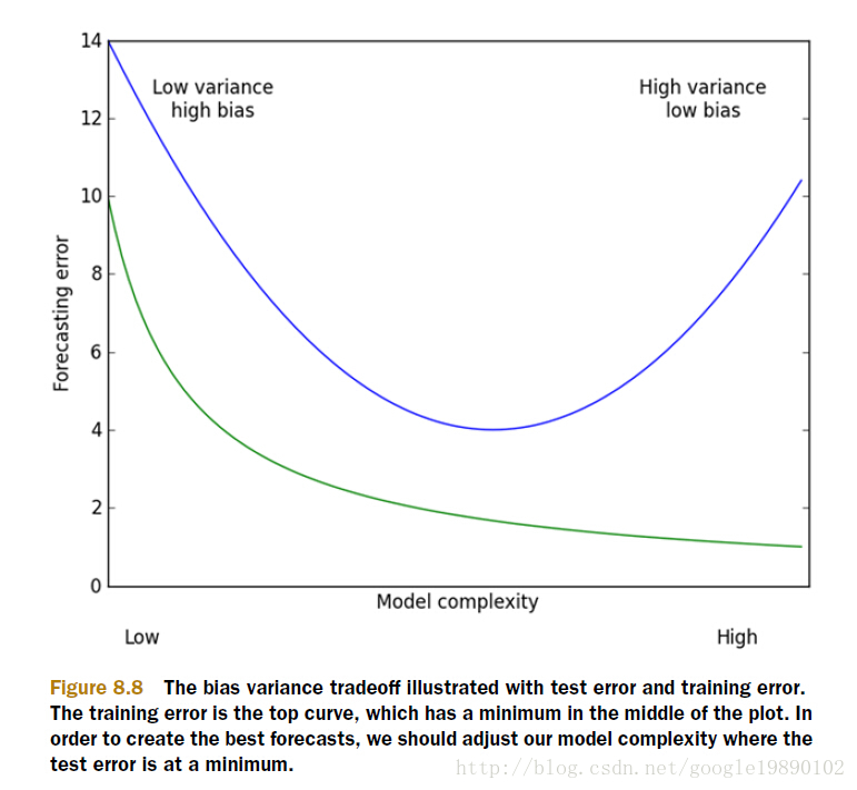

(摘自:机器学习实战)

方差指的是模型之间的差异,而偏差指的是模型预测值和数据之间的差异。我们需要找到方差和偏差的折中。

二、岭回归的概念

    在进行特征选择时,一般有三种方式:

  • 子集选择
  • 收缩方式(Shrinkage method),又称为正则化(Regularization)。主要包括岭回归和lasso回归。
  • 维数缩减
    岭回归(Ridge Regression)是在平方误差的基础上增加正则项

,

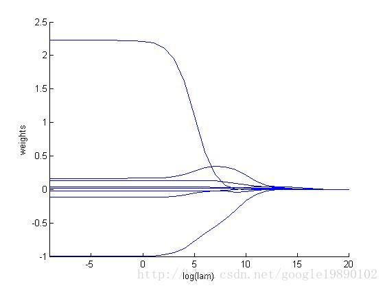
通过确定的值可以使得在方差和偏差之间达到平衡:随着的增大,模型方差减小而偏差增大。

    对求导,结果为


令其为0,可求得的值:


三、实验的过程

    我们去探讨一下取不同的对整个模型的影响。


和其他线性模型一样,Ridge 调用 fit 方法,参数为X,y,并且将线性模型拟合的系数 w 存到成员变量 coef_中。:

>>> from sklearn import linear_model
>>> clf = linear_model.Ridge (alpha = .5)
>>> clf.fit ([[0, 0], [0, 0], [1, 1]], [0, .1, 1]) 
Ridge(alpha=0.5, copy_X=True, fit_intercept=True, max_iter=None,
      normalize=False, random_state=None, solver='auto', tol=0.001)
>>> clf.coef_
array([ 0.34545455,  0.34545455])
>>> clf.intercept_ 
0.13636...
绘制岭系数正则化的函数
岭回归是本例中使用的估计量,美中衍射代表不同系数向量特征,在路径末端,alpha趋于零,解趋于普通最小二乘法,系数表现出现很大的震荡
../../_images/plot_ridge_path_001.png
# Author: Fabian Pedregosa -- <fabian.pedregosa@inria.fr>
# License: BSD 3 clauseprint(__doc__)import numpy as np
import matplotlib.pyplot as plt
from sklearn import linear_model# X is the 10x10 Hilbert matrix 希尔伯特矩阵
X = 1. / (np.arange(1, 11) + np.arange(0, 10)[:, np.newaxis])
y = np.ones(10)###############################################################################
# Compute paths a为alpha 正则化系数,通过便利-10 到 -2之间200个系数,来寻找最佳系数n_alphas = 200
alphas = np.logspace(-10, -2, n_alphas)
clf = linear_model.Ridge(fit_intercept=False)coefs = []
for a in alphas:clf.set_params(alpha=a)clf.fit(X, y)coefs.append(clf.coef_)###############################################################################
# Display resultsax = plt.gca()
ax.set_color_cycle(['b', 'r', 'g', 'c', 'k', 'y', 'm'])ax.plot(alphas, coefs)
ax.set_xscale('log')
ax.set_xlim(ax.get_xlim()[::-1])  # reverse axis
plt.xlabel('alpha')
plt.ylabel('weights')
plt.title('Ridge coefficients as a function of the regularization')
plt.axis('tight')
plt.show()

 
   class sklearn.linear_model.RidgeClassifier(alpha=1.0fit_intercept=Truenormalize=Falsecopy_X=Truemax_iter=Nonetol=0.001class_weight=Nonesolver='auto'random_state=None)[source]

Classifier using Ridge regression.

Read more in the User Guide.

Parameters:

alpha : float

Regularization strength; must be a positive float. Regularization improves the conditioning of the problem and reduces the variance of the estimates. Larger values specify stronger regularization. Alpha corresponds to C^-1 in other linear models such as LogisticRegression or LinearSVC.

class_weight : dict or ‘balanced’, optional

Weights associated with classes in the form {class_label: weight}. If not given, all classes are supposed to have weight one.

The “balanced” mode uses the values of y to automatically adjust weights inversely proportional to class frequencies in the input data as n_samples / (n_classes * np.bincount(y))

copy_X : boolean, optional, default True

If True, X will be copied; else, it may be overwritten.

fit_intercept : boolean

Whether to calculate the intercept for this model. If set to false, no intercept will be used in calculations (e.g. data is expected to be already centered).

max_iter : int, optional

Maximum number of iterations for conjugate gradient solver. The default value is determined by scipy.sparse.linalg.

normalize : boolean, optional, default False

If True, the regressors X will be normalized before regression. This parameter is ignored when fit_intercept is set to False. When the regressors are normalized, note that this makes the hyperparameters learnt more robust and almost independent of the number of samples. The same property is not valid for standardized data. However, if you wish to standardize, please use preprocessing.StandardScaler before calling fit on an estimator with normalize=False.

solver : {‘auto’, ‘svd’, ‘cholesky’, ‘lsqr’, ‘sparse_cg’, ‘sag’}

Solver to use in the computational routines:

  • ‘auto’ chooses the solver automatically based on the type of data.

  • ‘svd’ uses a Singular Value Decomposition of X to compute the Ridge coefficients. More stable for singular matrices than ‘cholesky’.

  • ‘cholesky’ uses the standard scipy.linalg.solve function to obtain a closed-form solution.

  • ‘sparse_cg’ uses the conjugate gradient solver as found in scipy.sparse.linalg.cg. As an iterative algorithm, this solver is more appropriate than ‘cholesky’ for large-scale data (possibility to set tol and max_iter).

  • ‘lsqr’ uses the dedicated regularized least-squares routine scipy.sparse.linalg.lsqr. It is the fastest but may not be available in old scipy versions. It also uses an iterative procedure.

  • ‘sag’ uses a Stochastic Average Gradient descent. It also uses an iterative procedure, and is faster than other solvers when both n_samples and n_features are large.

    New in version 0.17: Stochastic Average Gradient descent solver.

tol : float

Precision of the solution.

random_state : int seed, RandomState instance, or None (default)

The seed of the pseudo random number generator to use when shuffling the data. Used in ‘sag’ solver.

Attributes:

coef_ : array, shape (n_features,) or (n_classes, n_features)

Weight vector(s).

intercept_ : float | array, shape = (n_targets,)

Independent term in decision function. Set to 0.0 if fit_intercept = False.

n_iter_ : array or None, shape (n_targets,)

Actual number of iterations for each target. Available only for sag and lsqr solvers. Other solvers will return None.

See also


RidgeRidgeClassifierCV

Notes

For multi-class classification, n_class classifiers are trained in a one-versus-all approach. Concretely, this is implemented by taking advantage of the multi-variate response support in Ridge.

Methods

decision_function(X)Predict confidence scores for samples.
fit(X, y[, sample_weight])Fit Ridge regression model.
get_params([deep])Get parameters for this estimator.
predict(X)Predict class labels for samples in X.
score(X, y[, sample_weight])Returns the mean accuracy on the given test data and labels.
set_params(\*\*params)Set the parameters of this estimator.
__init__(alpha=1.0fit_intercept=Truenormalize=Falsecopy_X=Truemax_iter=Nonetol=0.001class_weight=Nonesolver='auto'random_state=None)[source]
decision_function(X)[source]

Predict confidence scores for samples.

The confidence score for a sample is the signed distance of that sample to the hyperplane.

Parameters:

X : {array-like, sparse matrix}, shape = (n_samples, n_features)

Samples.

Returns:

array, shape=(n_samples,) if n_classes == 2 else (n_samples, n_classes) :

Confidence scores per (sample, class) combination. In the binary case, confidence score for self.classes_[1] where >0 means this class would be predicted.

fit(Xysample_weight=None)[source]

Fit Ridge regression model.

Parameters:

X : {array-like, sparse matrix}, shape = [n_samples,n_features]

Training data

y : array-like, shape = [n_samples]

Target values

sample_weight : float or numpy array of shape (n_samples,)

Sample weight.

New in version 0.17: sample_weight support to Classifier.

Returns:

self : returns an instance of self.

get_params(deep=True)[source]

Get parameters for this estimator.

Parameters:

deep : boolean, optional

If True, will return the parameters for this estimator and contained subobjects that are estimators.

Returns:

params : mapping of string to any

Parameter names mapped to their values.

predict(X)[source]

Predict class labels for samples in X.

Parameters:

X : {array-like, sparse matrix}, shape = [n_samples, n_features]

Samples.

Returns:

C : array, shape = [n_samples]

Predicted class label per sample.

score(Xysample_weight=None)[source]

Returns the mean accuracy on the given test data and labels.

In multi-label classification, this is the subset accuracy which is a harsh metric since you require for each sample that each label set be correctly predicted.

Parameters:

X : array-like, shape = (n_samples, n_features)

Test samples.

y : array-like, shape = (n_samples) or (n_samples, n_outputs)

True labels for X.

sample_weight : array-like, shape = [n_samples], optional

Sample weights.

Returns:

score : float

Mean accuracy of self.predict(X) wrt. y.

set_params(**params)[source]

Set the parameters of this estimator.

The method works on simple estimators as well as on nested objects (such as pipelines). The latter have parameters of the form <component>__<parameter> so that it’s possible to update each component of a nested object.

文章参考:http://blog.csdn.net/google19890102/article/details/27228279

这篇关于scikit-learn linearRegression 1.1.2 岭回归的文章就介绍到这儿,希望我们推荐的文章对编程师们有所帮助!


http://www.chinasem.cn/article/957526

相关文章

usaco 1.1 Broken Necklace(DP)

直接上代码 接触的第一道dp ps.大概的思路就是 先从左往右用一个数组在每个点记下蓝或黑的个数 再从右到左算一遍 最后取出最大的即可 核心语句在于: 如果 str[i] = 'r'  ,   rl[i]=rl[i-1]+1, bl[i]=0 如果 str[i] = 'b' ,  bl[i]=bl[i-1]+1, rl[i]=0 如果 str[i] = 'w',  bl[i]=b

【WebGPU Unleashed】1.1 绘制三角形

一部2024新的WebGPU教程,作者Shi Yan。内容很好,翻译过来与大家共享,内容上会有改动,加上自己的理解。更多精彩内容尽在 dt.sim3d.cn ,关注公众号【sky的数孪技术】,技术交流、源码下载请添加微信号:digital_twin123 在 3D 渲染领域,三角形是最基本的绘制元素。在这里,我们将学习如何绘制单个三角形。接下来我们将制作一个简单的着色器来定义三角形内的像素

✨机器学习笔记(二)—— 线性回归、代价函数、梯度下降

1️⃣线性回归(linear regression) f w , b ( x ) = w x + b f_{w,b}(x) = wx + b fw,b​(x)=wx+b 🎈A linear regression model predicting house prices: 如图是机器学习通过监督学习运用线性回归模型来预测房价的例子,当房屋大小为1250 f e e t 2 feet^

用Python实现时间序列模型实战——Day 14: 向量自回归模型 (VAR) 与向量误差修正模型 (VECM)

一、学习内容 1. 向量自回归模型 (VAR) 的基本概念与应用 向量自回归模型 (VAR) 是多元时间序列分析中的一种模型,用于捕捉多个变量之间的相互依赖关系。与单变量自回归模型不同,VAR 模型将多个时间序列作为向量输入,同时对这些变量进行回归分析。 VAR 模型的一般形式为: 其中: ​ 是时间  的变量向量。 是常数向量。​ 是每个时间滞后的回归系数矩阵。​ 是误差项向量,假

Learn ComputeShader 09 Night version lenses

这次将要制作一个类似夜视仪的效果 第一步就是要降低图像的分辨率, 这只需要将id.xy除上一个数字然后再乘上这个数字 可以根据下图理解,很明显通过这个操作在多个像素显示了相同的颜色,并且很多像素颜色被丢失了,自然就会有降低分辨率的效果 效果: 但是这样图像太锐利了,我们加入噪声去解决这个问题 [numthreads(8, 8, 1)]void CSMain(uint3 id

深度学习与大模型第3课:线性回归模型的构建与训练

文章目录 使用Python实现线性回归:从基础到scikit-learn1. 环境准备2. 数据准备和可视化3. 使用numpy实现线性回归4. 使用模型进行预测5. 可视化预测结果6. 使用scikit-learn实现线性回归7. 梯度下降法8. 随机梯度下降和小批量梯度下降9. 比较不同的梯度下降方法总结 使用Python实现线性回归:从基础到scikit-learn 线性

【python因果推断库11】工具变量回归与使用 pymc 验证工具变量4

目录  Wald 估计与简单控制回归的比较 CausalPy 和 多变量模型 感兴趣的系数 复杂化工具变量公式  Wald 估计与简单控制回归的比较 但现在我们可以将这个估计与仅包含教育作为控制变量的简单回归进行比较。 naive_reg_model, idata_reg = make_reg_model(covariate_df.assign(education=df[

什么是GPT-3的自回归架构?为什么GPT-3无需梯度更新和微调

文章目录 知识回顾GPT-3的自回归架构何为自回归架构为什么架构会影响任务表现自回归架构的局限性与双向模型的对比小结 为何无需梯度更新和微调为什么不需要怎么做到不需要 🍃作者介绍:双非本科大四网络工程专业在读,阿里云专家博主,专注于Java领域学习,擅长web应用开发,目前开始人工智能领域相关知识的学习 🦅个人主页:@逐梦苍穹 📕所属专栏:人工智能 🌻gitee地址:x

1.1 Avtivity的生命周期全面分析

本文将Activity的生命周期分为两部分内容,一部分是典型情况下的生命周期,另一部分是异常情况下的生命周期。所谓典型情况下的生命周期,是指在有用户参与的情况下,Activity所经过的生命周期的改变;而异常情况下的生命周期是指在Activity被系统回收或者由于当前设备的Configuration发生改变从而导致Activity被销毁重建,异常情况下的生命周期的关注点和典型情况下略有不同。 1

回归预测 | MATLAB实现PSO-LSTM(粒子群优化长短期记忆神经网络)多输入单输出

回归预测 | MATLAB实现PSO-LSTM(粒子群优化长短期记忆神经网络)多输入单输出 目录 回归预测 | MATLAB实现PSO-LSTM(粒子群优化长短期记忆神经网络)多输入单输出预测效果基本介绍模型介绍PSO模型LSTM模型PSO-LSTM模型 程序设计参考资料致谢 预测效果 Matlab实现PSO-LSTM多变量回归预测 1.input和outpu