方程自己解（3）——deepXDE解Burgers方程

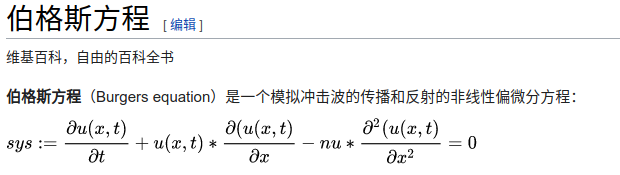
1. what‘s Burgers equation

2. Solve Burgers equation by DeepXDE

Burgers equation:
$$\frac{du}{dt}+u\frac{du}{dx}=v\frac{d^{2}u}{d{x}^2},x\in [-1,1],t\in [0,1]\text{\hspace{1em}(1)}$$
Dirichlet boundary conditions and initial conditions
$$u(-1,t)=u(1,t)=0,u(x,0)=-sin(\pi x)$$
reference solution: here

import deepxde as dde
import numpy as np
import matplotlib.pyplot as plt 

def gen_testdata():""" generate test data with react synthetic result"""data = np.load("../deepxde/examples/dataset/Burgers.npz")t, x, exact = data["t"], data["x"], data["usol"].Txx, tt = np.meshgrid(x, t)X = np.vstack((np.ravel(xx), np.ravel(tt))).Ty = exact.flatten()[:, None]return X, ydef pde(x, y):dy_x = dde.grad.jacobian(y, x, i=0, j=0)dy_t = dde.grad.jacobian(y, x, i=0, j=1)dy_xx = dde.grad.hessian(y, x, i=0, j=0)return dy_t + y * dy_x - 0.01 / np.pi * dy_xx

geom = dde.geometry.Interval(-1, 1)
timedomain = dde.geometry.TimeDomain(0, 0.99)
# define Geometry and time domain,and we combine both the domain using GeometryXTime
geomtime = dde.geometry.GeometryXTime(geom, timedomain) 
bc = dde.DirichletBC(geomtime, lambda x: 0, lambda _, on_boundary: on_boundary)
ic = dde.IC(geomtime, lambda x: -np.sin(np.pi * x[:, 0:1]), lambda _, on_initial: on_initial
)

data = dde.data.TimePDE(geomtime, pde, [bc, ic], num_domain=2540, num_boundary=80, num_initial=160
)

net = dde.maps.FNN([2] + [20] * 3 + [1], "tanh", "Glorot normal")
model = dde.Model(data, net)

# Now, we have the PDE problem and the network. We bulid a Model and choose the optimizer and learning rate
model.compile("adam", lr=1e-3)# We then train the model for 15000 iterations:
model.train(epochs=15000)
# After we train the network using Adam, we continue to train the network using L-BFGS to achieve a smaller loss:
model.compile("L-BFGS")
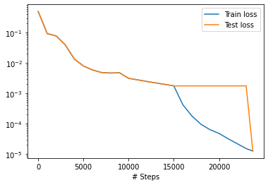
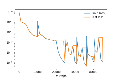
losshistory, train_state = model.train()dde.saveplot(losshistory, train_state, issave=True, isplot=True)

X, y_true = gen_testdata()
y_pred = model.predict(X)
f = model.predict(X, operator=pde)
print("Mean residual:", np.mean(np.absolute(f)))
print("L2 relative error:", dde.metrics.l2_relative_error(y_true, y_pred))
np.savetxt("test.dat", np.hstack((X, y_true, y_pred)))

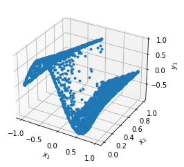
Mean residual: 0.033188015
L2 relative error: 0.17063112901692742

%matplotlib notebook
import matplotlib.pyplot as plt
fig = plt.figure()
ax = plt.axes(projection='3d')
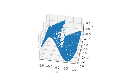
ax.plot3D(X[:,0].reshape(-1),X[:,1].reshape(-1),y_true.reshape(-1),'red')
ax.plot3D(X[:,0].reshape(-1),X[:,1].reshape(-1),y_pred.reshape(-1),'blue',alpha=0.5)
plt.show()

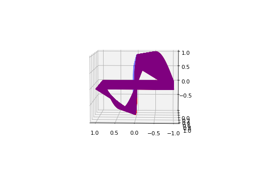
2. Burgers RAR

函数定义和上面是一样的，这里地RAR地目的在于不断减小函数拟合地误差到一个指定地误差范围之下。控制误差的大小。

import deepxde as dde
import numpy as npdef gen_testdata():data = np.load("../deepxde/examples/dataset/Burgers.npz")t, x, exact = data["t"], data["x"], data["usol"].Txx, tt = np.meshgrid(x, t)X = np.vstack((np.ravel(xx), np.ravel(tt))).Ty = exact.flatten()[:, None]return X, ydef pde(x, y):dy_x = dde.grad.jacobian(y, x, i=0, j=0)dy_t = dde.grad.jacobian(y, x, i=0, j=1)dy_xx = dde.grad.hessian(y, x, i=0, j=0)return dy_t + y * dy_x - 0.01 / np.pi * dy_xxgeom = dde.geometry.Interval(-1, 1)
timedomain = dde.geometry.TimeDomain(0, 0.99)
geomtime = dde.geometry.GeometryXTime(geom, timedomain)bc = dde.DirichletBC(geomtime, lambda x: 0, lambda _, on_boundary: on_boundary)
ic = dde.IC(geomtime, lambda x: -np.sin(np.pi * x[:, 0:1]), lambda _, on_initial: on_initial
)data = dde.data.TimePDE(geomtime, pde, [bc, ic], num_domain=2500, num_boundary=100, num_initial=160
)
net = dde.maps.FNN([2] + [20] * 3 + [1], "tanh", "Glorot normal")
model = dde.Model(data, net)model.compile("adam", lr=1.0e-3)
model.train(epochs=10000)
model.compile("L-BFGS")
model.train()

X = geomtime.random_points(100000)
err = 1
while err > 0.005:f = model.predict(X, operator=pde)err_eq = np.absolute(f)err = np.mean(err_eq)print("Mean residual: %.3e" % (err))x_id = np.argmax(err_eq)print("Adding new point:", X[x_id], "\n")data.add_anchors(X[x_id])early_stopping = dde.callbacks.EarlyStopping(min_delta=1e-4, patience=2000)model.compile("adam", lr=1e-3)model.train(epochs=10000, disregard_previous_best=True, callbacks=[early_stopping])model.compile("L-BFGS")losshistory, train_state = model.train()
dde.saveplot(losshistory, train_state, issave=True, isplot=True)X, y_true = gen_testdata()
y_pred = model.predict(X)
print("L2 relative error:", dde.metrics.l2_relative_error(y_true, y_pred))
np.savetxt("test.dat", np.hstack((X, y_true, y_pred)))

L2 relative error: 0.009516824350586142

%matplotlib notebook
import matplotlib.pyplot as plt
fig = plt.figure()
ax = plt.axes(projection='3d')
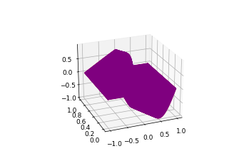
ax.plot3D(X[:,0].reshape(-1),X[:,1].reshape(-1),y_true.reshape(-1),'red')
ax.plot3D(X[:,0].reshape(-1),X[:,1].reshape(-1),y_pred.reshape(-1),'blue',alpha=0.5)
plt.show()

4. summary

1. 迭代更多的次数，在方程拟合的过程中可能会获得更好的结果，但是也可能陷入一些局部最优值，LR的影响还是挺大的
2. 两次对比，第二次固定一个最大容忍误差值进行判断，最终得到一个误差非常小的模型。这对于PINN的训练而言似乎是一个可行的方案，因为一般不存在过拟合的问题。
3. 注意我们的PINN方法是一个无监督学习过程。
4. 对于二维的Burgers方程的训练和预测速度都还是非常快的，尽管我的GPU非常普通。暂时对于我是可以容忍的！！！