[论文精读]BrainGNN: Interpretable Brain Graph Neural Network for fMRI Analysis

本文主要是介绍[论文精读]BrainGNN: Interpretable Brain Graph Neural Network for fMRI Analysis，希望对大家解决编程问题提供一定的参考价值，需要的开发者们随着小编来一起学习吧！

论文原文：BrainGNN: Interpretable Brain Graph Neural Network for fMRI Analysis - ScienceDirect

英文是纯手打的！论文原文的summarizing and paraphrasing。可能会出现难以避免的拼写错误和语法错误，若有发现欢迎评论指正！文章偏向于笔记，谨慎食用！

1. 一些概念

1.1. 嵌入

1.2. 池化正则图神经网络

1.3. 省流总结图

2. 原文逐段精读

2.1. Introduction

2.2. BrainGNN

2.2.1. Notations

2.2.2. Architecture overview

2.2.3. Layers in BrainGNN

2.2.4. Loss functions

2.2.5. Interpretation from BrainGNN

2.3. Experiments and results

2.3.1. Datasets

2.3.2. Experimental setup

2.3.3. Hyperparameter discussion and ablation study

2.3.4. Comparison with baseline methods

2.3.5. Interpretability of BrainGNN

2.4. Discussion

2.4.1. The model

2.4.2. Limitation and future work

2.5. Conclusions

3. Reference List

1. 一些概念

1.1. 嵌入

嵌入是用连续向量表示离散变量，且是有监督学习。在监督学习中学习合适的权重以最小化损失函数。它能用低维向量表示数据并保留数据的特征，且很容易找到临近或相似的概念。

1.2. 池化正则图神经网络

文中的表述是Pooling Regularized Graph Neural Network. 并没有在网上搜到一样的，只搜到了Regularized Pooling (Otsuzuki et al., 2020). 其中Otsuzuki等人表示最大化池化过于杂乱无序而正则化池化平滑有序（颜色越深值越大，箭头为取的池化值与中心点的距离）

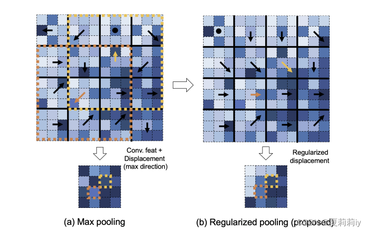
然后文章设滑窗是步距为s1的n*n核，垂直方向能滑动I次，水平能滑动J次。因此可以定义池化核的矩阵（二维数组）。然后可以用 $\Delta _{i,j}$ 来确定核中心到最大值的方向（一个向量）。用相邻位移方向正则化位移方向。公式如下：

$\widetilde{\Delta}_{i,j}=\frac{1}{w^2}\sum_{(p,q)\in P_{ij}}\Delta_{p,q}$

其中w为平滑窗口的大小，从而得到新的位移方向。若算出来的位移非整数，如n为奇数则将其四舍五入到整数，如n为偶数则要让其不为零地四舍五入？

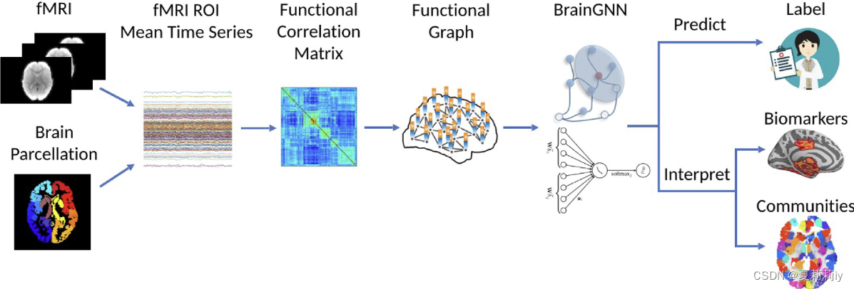
1.3. 省流总结图

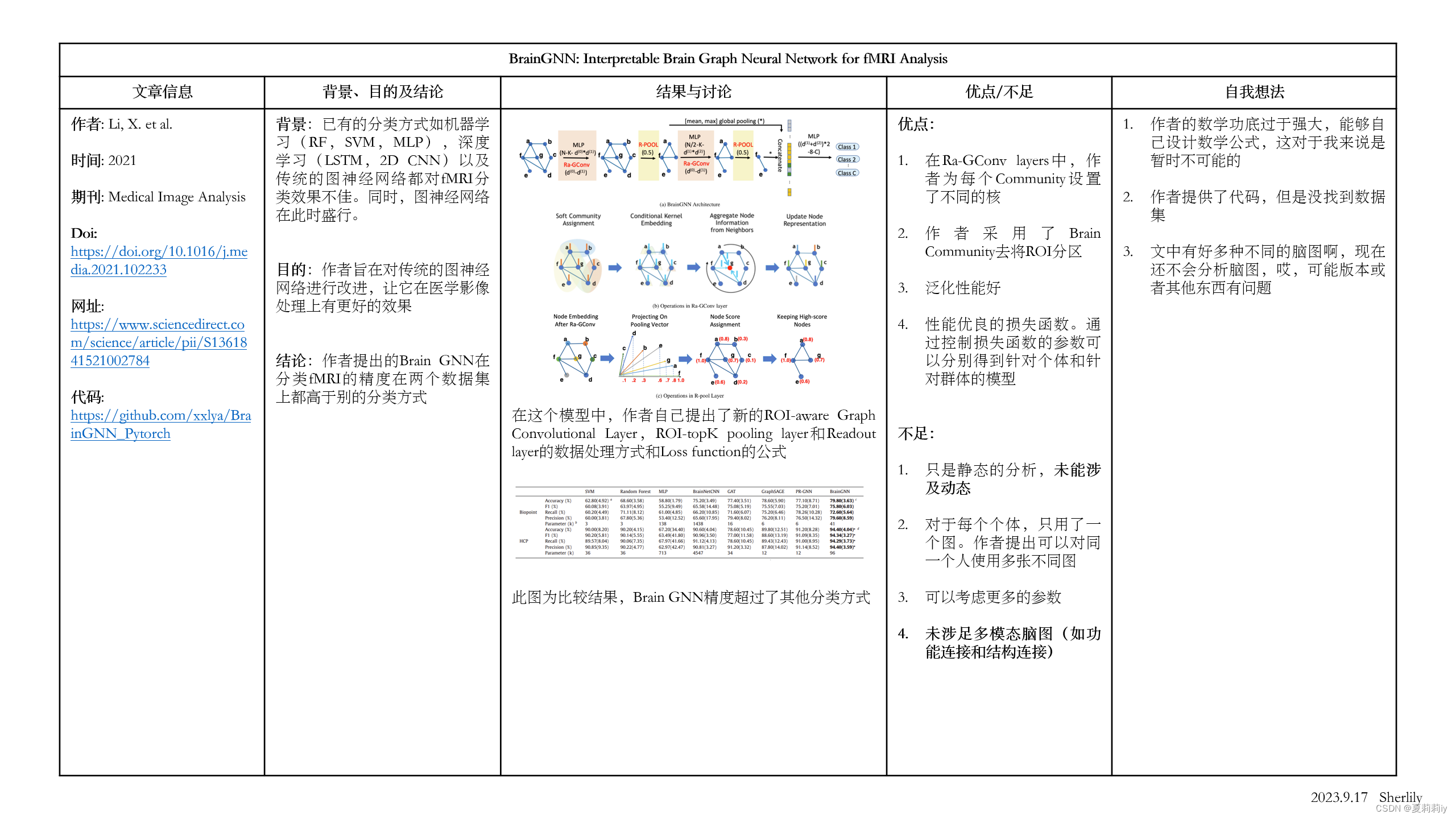
2. 原文逐段精读

2.1. Introduction

（1）Regarding pictures in fMRI as graphs makes a mighty advance in history. What is more, in this model, nodes reperesent brain regions of interest (ROIs) while edges represent functional connectivity.

atlas n.地图集 parcellation n.分割 salient adj.显著的，突出的，最重要的

（2）Traditional graph firstly extracts features and then anaylse them. Clustering ROIs into highly connected communities (这是啥啊为什么搜不到) is an effective way to reduce dimensionality brought by fMRI data. Moreover, error in extraction causes salient deviation in analysis.

（3）作者说大多数现存GNN在不同的实例中的节点没有对应关系上？？？？然后举例说比如社交网络和蛋白质网络（啥意思，社交网络的节点为啥没有对应关系？）又及，为什么作者说不同的节点是相同的嵌入这样不好？按理来说每个节点不是有自己的向量吗哪里是相同的嵌入？啥是嵌入？

（4）Different form those who set subject as node, authors model one brain as a graph. Besides, they enhance the interpretability by adding pooling scores with similarity.

（5）Mentions Pooling Regularized Graph Neural Network.

2.2. BrainGNN

2.2.1. Notations

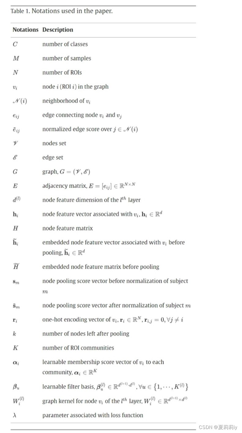
Undirected weighted graph is uesed in this paper, and G can be represented as matrix $H=\left[\mathbf{h}_1,\cdots,\mathbf{h}_N\right]^\top$ where h is the feature vector of v. As every existing edge, define e∈R and e＞0. For any edge is not existed, set it by 0. Then, make a adjacency matrix.

2.2.2. Architecture overview

（1）Classification:

①embedding nodes in low dimension and coarsening or pooling them

②then, put all them in MLP

③train convolutional and pooling layers

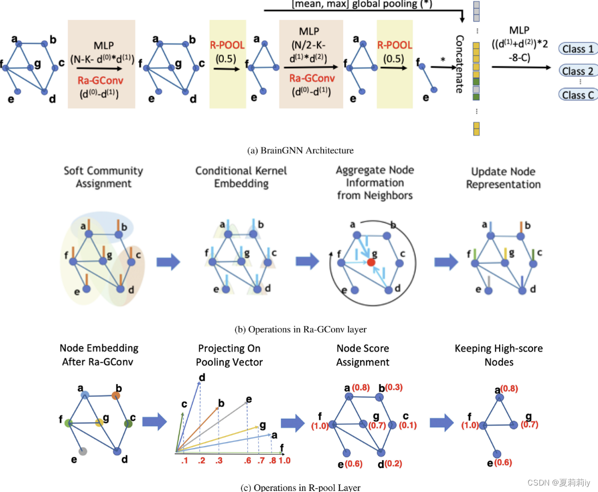
④ (a) shows the structure. (b) presents how to extract feature. (c) ⭐ignore nodes which are low in projection value

recursively adv.递归地 aggregate adj.总数的 n.总数，合计 vt.合计

（2）Graph convolutional layer use edge feature????（但是上面的图是用的节点啊）(看下面公式感觉边和节点都要用)

（3）Propagation model is as follows:

$\widetilde{\mathbf{h}}_i^{(l+1)}=\text{relu}\left(W_i^{(l)}\mathbf{h}_i^{(l)}+\sum_{j\in\mathcal{N}^{(l)}(i)}e_{ij}^{(l)}W_j^{(l)}\mathbf{h}_j^{(l)}\right)$

where W denotes the parameters which need to be learned. ⭐Furthermore, to control output scale, it is necessary to normalize edge feature. Weights normalization is as follows:

$e_{ij}^{(l)}=e_{ij}^{(l)}/\sum_{j\in\mathcal{N}^{(l)}(i)}e_{ij}^{(l)}.$

（4）Nodes are mostly grouped or pruned to subgraph, which could reduce size of graph

prune v.修剪

（5）Readout is combine all h together in one vector z

2.2.3. Layers in BrainGNN

（1）ROI-aware Graph Convolutional Layer

①The model learns different embedding weights. Secondly, they assume ROIs which connected closely impact more on each other. There is function of ROI-aware graph convolutional layer (Ra-GConv):

$\mathrm{vec}\left(W_i^{(l)}\right)=f_{MLP}^{(l)}\left(\mathbf{r}_i\right)=\Theta_2^{(l)}\mathrm{relu}\left(\Theta_1^{(l)}\mathbf{r}_i\right)+\mathbf{b}^{(l)}$

where W is a linear combination of a set of basis functions, and basis functions denote community. r denotes one-hot encoding vectors of v in $d^{(l+1)}\cdot d^{(l)}$ dimension(I guess it is a integer), and reshapes output to a $d^{(l+1)} \times d^{(l)}$ matrix W. Θ denotes parameters. b is the bias in MLP.

②Every brain graph presents same manner. Thus brain nodes between different person are able to align. However, convolutional embedding is independent of how to order those graphs. Besides, one hot encoding is used for ROI locating information. Then, r, vector with N dimension, 1 represents the $i^{th}$ entry and 0 represents the other entries（什么其他entry？为什么不是没有entry？）.

Assume

$\Theta_1^{(l)}=\left[\boldsymbol{\alpha}_1^{(l)},\cdots,\boldsymbol{\alpha}_{N^{(l)}}^{(l)}\right]$ where N is the number of ROIs in the $l^{th}$ layer, and $\boldsymbol{\alpha}_i^{(l)}=\left[\alpha_{i1}^{(l)},\cdots,\alpha_{iK^{(l)}}^{(l)}\right]^\top\in\mathbb{R}^{K^{(l)}}$ , $\forall i\in\begin{Bmatrix}1,\cdots,N^{(l)}\end{Bmatrix}$ with K can be seen as the number of clustered communities for the N ROIs.

Also

$\Theta_2^{(l)}=\left[\boldsymbol{\beta}_1^{(l)},\cdots,\boldsymbol{\beta}_{K^{(l)}}^{(l)}\right]$ where $\boldsymbol{\beta}_u^{(l)}\in\mathbb{R}^{d^{(l+1)}\cdot d^{(l)}}$ , $\forall u\in\left\{1,\cdots,K^{(l)}\right\}$

Though this, function

$\mathrm{vec}\left(W_i^{(l)}\right)=f_{MLP}^{(l)}\left(\mathbf{r}_i\right)=\Theta_2^{(l)}\mathrm{relu}\left(\Theta_1^{(l)}\mathbf{r}_i\right)+\mathbf{b}^{(l)}$

can be rewritten as

$\operatorname{vec}\left(W_i^{(l)}\right)=\sum_{u=1}^{K^{(l)}}\left(\alpha_{iu}^{(l)}\right)^+\boldsymbol{\beta}_u^{(l)}+\boldsymbol{b}^{(l)}$

where $\left(\alpha_{iu}^{(l)}\right)^+$ denotes coordinates which stores positive ROI result after ReLU regularization. Also, see $\left\{\boldsymbol{\beta}_{u}^{(l)}:j=1,\cdots,K^{(l)}\right\}$ as a basis. Most of the time, number of ROI communities is far less than the number of ROIs. Besides, embedding separating kernal to each ROI. Lastly, ROIs in same community embedded by similar kernals.

Deduction by myself lies here:

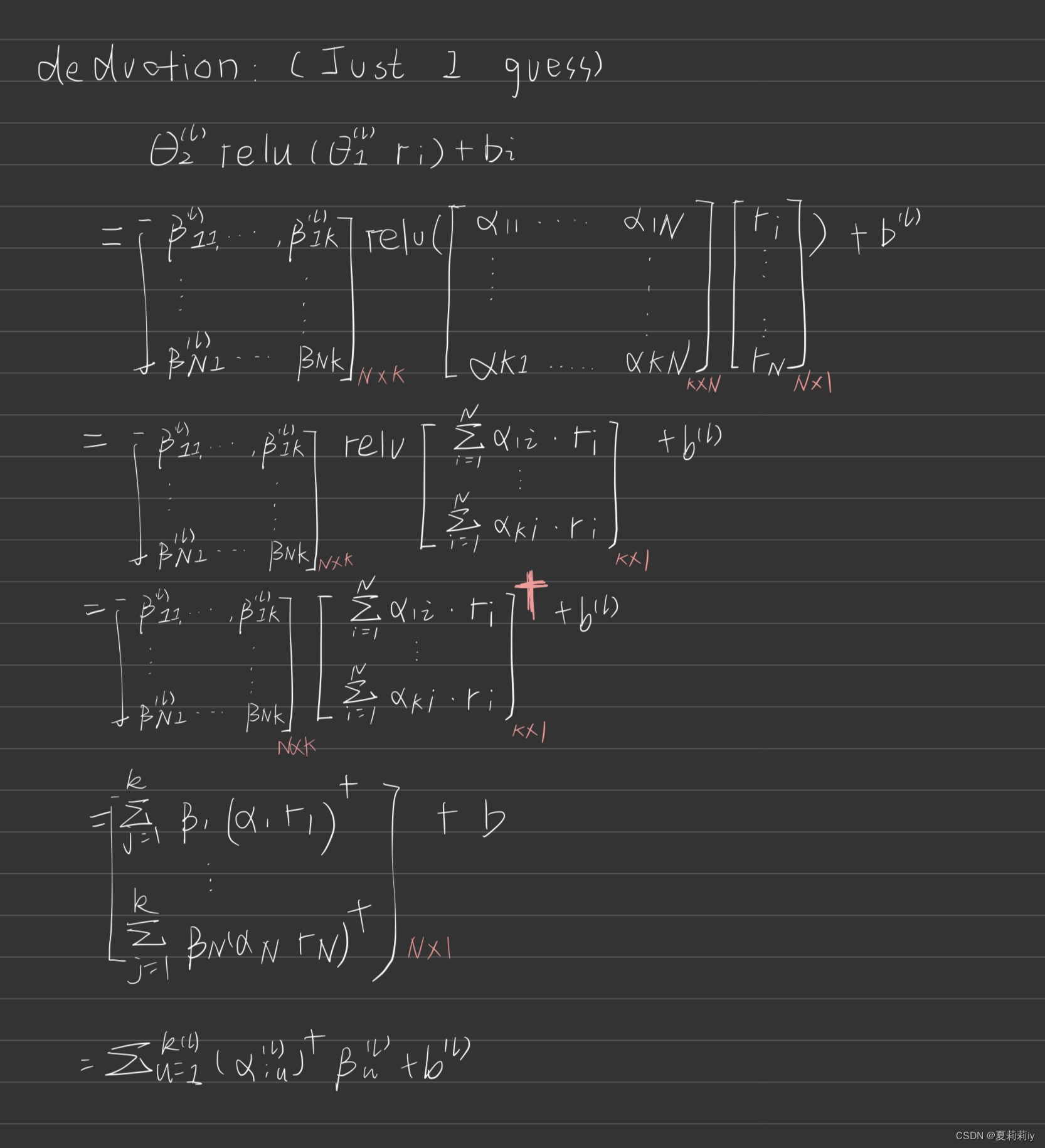
③Additionaly, authors mention the feature values of nodes are multiplied by the weights of edges, so surrounding nodes can also have an impact on them

（2）ROI-topK pooling layer

①For some ROIs show more indicative character to predict neurological disorders, they should be kept in dimension reduction while other nosiy nodes should be pruned.

②Functions in pooling layer show below:

$\begin{aligned} &\mathbf{s}^{(l)}&& =\widetilde{H}^{(l+1)}\mathbf{w}^{(l)}\left/\left\|\mathbf{w}^{(l)}\right\|_2\right. \\ &\mathbf{\tilde{s}}^{(l)}&& =\left(\mathbf{s}^{(l)}-\mu\left(\mathbf{s}^{(l)}\right)\right)/\sigma\left(\mathbf{s}^{(l)}\right) \\ & i && =\mathrm{top}k(\mathbf{\tilde{s}}^{(l)},k) \\ &H^{(l+1)}&& =\left(\widetilde{H}^{(l+1)}\odot\text{sigmoid}\left(\tilde{\mathbf{s}}^{(l)}\right)\right)_{\mathbf{i},:} \\ &E^{(l+1)}&& =E_{\mathbf{i},\mathbf{i}}^{(l)}. \end{aligned}$

where $\left\|\cdot\right\|$ denotes L2 norm (calculate the sum of squares for each element of a vector and then root out the entire vector);

function μ() calculates the mean value of its inside parameter;

function σ() calculates the standard deviation value of its inside parameter;

function topl() finds the largest k elements in $\tilde{s}$ (这绕口英语读半天，我觉得就是在向量 $\tilde{s}$ 里面找最大的k个元素);

Hadamard product⊙矩阵是对应元素相乘，和矩阵的点乘和叉乘都不一样（以防写英语以后看不懂描述了，这里改用中文）不过我真的觉得很炸裂的是按照2.2.1的表H不是矩阵，s不是向量吗怎么求哈达玛积啊难道和右下角的行索引有关吗？但是就算行索引了s不是列向量吗？？？？

参考代码（不知道是不是这里），但是也很炸裂的是把x降维了

 weight = self.nn(pseudo).view(-1, self.in_channels, self.out_channels)if torch.is_tensor(x):"""这里出现了哈达玛积，就是矩阵乘法"""x = torch.matmul(x.unsqueeze(1), weight).squeeze(1)else:x = (None if x[0] is None else torch.matmul(x[0].unsqueeze(1), weight).squeeze(1),None if x[1] is None else torch.matmul(x[1].unsqueeze(1), weight).squeeze(1))

$(\cdot)_{\mathbf{i},\mathbf{j}}$ denotes indexing, which i is by row and j is by column

idiomatically adv. 惯用地

（3）Readout layer

The matrix after convolution needs to be flatten. The function authors put forward is:

$\mathbf{z}^{(l)}=\max H^{(l)}\|\max H^{(l)}$

where || denotes concatenation

这里原本是没有读懂的，因为不知道||到底表达什么样的串联，因此查阅代码：

"""extracted from braingnn.py""""""这是作者给的requirements.txt下载的"""
from torch_geometric.nn import global_mean_pool as gap, global_max_pool as gmp"""传播函数"""def forward(self, x, edge_index, batch, edge_attr, pos):x = self.conv1(x, edge_index, edge_attr, pos)x, edge_index, edge_attr, batch, perm, score1 = self.pool1(x, edge_index, edge_attr, batch)pos = pos[perm]"""这里就能很明显看出来用的torch.cat以列为主方向连接，这里是z=mean H||max H的列方向连接"""x1 = torch.cat([gmp(x, batch), gap(x, batch)], dim=1)edge_attr = edge_attr.squeeze()edge_index, edge_attr = self.augment_adj(edge_index, edge_attr, x.size(0))x = self.conv2(x, edge_index, edge_attr, pos)x, edge_index, edge_attr, batch, perm, score2 = self.pool2(x, edge_index,edge_attr, batch)x2 = torch.cat([gmp(x, batch), gap(x, batch)], dim=1)"""这是将所有z列方向连接，因此我揣测最后是长度为2*L的一维行向量"""x = torch.cat([x1,x2], dim=1)x = self.bn1(F.relu(self.fc1(x)))x = F.dropout(x, p=0.5, training=self.training)x = self.bn2(F.relu(self.fc2(x)))x= F.dropout(x, p=0.5, training=self.training)x = F.log_softmax(self.fc3(x), dim=-1)return x,self.pool1.weight,self.pool2.weight, torch.sigmoid(score1).view(x.size(0),-1), torch.sigmoid(score2).view(x.size(0),-1)

concretely adv. 具体地 concatenation n. 一系列相关联的事物(或事件)

（4）Putting layers together

①They use two-layer GNN block

②Each block follows a readout layer

2.2.4. Loss functions

（1）The paper sets classification loss function as:

$L_{ce}=-\frac{1}{M}\sum_{m=1}^{M}\sum_{c=1}^{C}y_{m,c}\log\left(\hat{y}_{m,c}\right)$

where $y_{m,c}$ is the ground truth, $\hat{y}_{m,c}$ is prediction by GNN

（2）While setting unit loss function as:

$L_{unit}^{(l)}=(\|\mathbf{w}^{(l)}\|_2-1)^2$

authors point out there is a potential unidentifiable issue in $\mathbf{s}^{(l)}=\widetilde{H}^{(l+1)}\mathbf{w}^{(l)}\left/\left\|\mathbf{w}^{(l)}\right\|_{2}\right.$ in that learnable parameter w can be scaled proportionally at will with no change of the s. For example, s will be the same as $\mathbf{s}^{(l)}=\widetilde{H}^{(l+1)}\mathbf{aw}^{(l)}\left/\left\|\mathbf{aw}^{(l)}\right\|_{2}\right.$ . ⭐Hence, change w to unit vector could avoid this problem.

scalar adj. 标量的，无向量的 n. 标量 identifiability n.可识别性

（3）And setting group-level consistency(GLC) loss function as:

$L_{GLC}=\sum_{c=1}^{C}\sum_{m,n\in\i_{c}}\left\|\mathbf{\tilde{s}}_m^{(1)}-\mathbf{\tilde{s}}_n^{(1)}\right\|^2 =2\sum_{c=1}^C\mathrm{Tr}\left(\left(S_c^{(1)}\right)^{\top}L_cS_c^{(1)}\right)$

where $\i_c=\{m:m=1,\cdots,M,y_{m,c}=1\}$ and $c=1,\cdots,C$ ;

$y_{m,c}=1$ means the $m^{th}$ instance belongs to class c;

$S_{c}^{(1)}=\left[\mathbf{\tilde{s}}_{m}^{(1)}:m\in\i_{c}\right]^{\top}\in\mathbb{R}^{\left |\i_{c} \right |\times N}$ belongs to class c;

$L_{c}=D_{c}-W_{c}$ which is a symmetric positive semidefinite matrix;

$W_{c}$ is a $\left |\i_{c}\right |$ -dimensional square matrix with all elements are 1;

$D_{c}$ is a $\left |\i_{c}\right |$ -dimensional square diagonal matrix with all elements are 1;

Group-level consistency is for finding corresponding between ROIs and subjects. 然后作者提到对于不同的H， $\tilde{\mathbf{s}}$ 可能和原始图形中的同一组节点并不对应。这是因为 $\tilde{\mathbf{s}}$ 是向量吗？而原始H是矩阵？Also,GLC only be used after the first pooling layer.

（4）Also, setting TopK pooling loss function as:

$\begin{aligned} &L_{TPK}^{(l)} &=-\frac{1}{M} &\sum_{m=1}^{M}\frac1{N^{(l)}}\left(\sum_{i=1}^{k}\log\left(\hat{s}_{m,i}^{(l)}\right)+\sum_{i=1}^{N^{(l)}-k}\log\left(1-\hat{s}_{m,i+k}^{(l)}\right)\right) \end{aligned}$

where $\hat{\mathbf{s}}_{m}^{(l)}=\left[\hat{s}_{m,1}^{(l)},\cdots,\hat{s}_{m,N^{(l)}}^{(l)}\right]$ is in a descending order;

The importance of brain ROI may vary for different individuals. Therefore, scores close to one and close to zero should be distinguished to significantly differentiate ROI.

（5）By screening and removing intermediate data through ablation experiments, significant regularization pooling scores are retained:

ablation n. 消融，磨蚀

（6）Finally, combine all loss functions:

$\begin{aligned}L_{total}=L_{ce}+\sum_{l=1}^LL_{unit}^{(l)}+\lambda_1\sum_{l=1}^LL_{TPK}^{(l)}+\lambda_2L_{GLC}\end{aligned}$

where λ is tunable hyper-parameter;

$l$ denotes the $l^{th}$ GNN block and $L$ is the total number of GNN blocks;

Meanwhile, by adjusting the hyper-parameter w, the magnitudes of $L_{unit}^{(l)}$ and $L_{ce}$ are the same

2.2.5. Interpretation from BrainGNN

（1）Community detection from convolutional layers

①Mentions how essential the community patterns are.

② $a_{iu}^{+}$ means ROI i which belongs to community u.

③Belonging relationship defines when $\alpha_{iu}>\mu\left(\boldsymbol{\alpha}_i^+\right)+\sigma\left(\boldsymbol{\alpha}_i^+\right)$ where $\{\boldsymbol{i}_u\subset\{1,\ldots,N\}:u=1,\ldots,K\}$

（2）Biomarker Detection from pooling layers

①TPK helps to dispart nodes

②GLC controls balance of group and individual. Through tuning $\lambda_{2}$ , with high for commonality and low for individuation, reseachers could focus on different part.

coefficient n.系数 adj.共同作用的

2.3. Experiments and results

2.3.1. Datasets

For classifying Autism Spectrum Disorder (ASD) and Healthy Control (HC) person, they give tasks on gambling, language, motor, relational, social, working memory (WM), and emotion. In this way, detect and decode related ROIs. Moreover, all this is based on Biopoint Autism Study Dataset (Biopoint) and Human Connectome Project (HCP) 900 Subject Release datasets with mutually independent.

（1）Biopoint dataset

①Task: watching biological motion with point-light

②Screen: removing head motion ＞ 0.5mm translation or ＞ 0.5° rotation takes 25% or more time.

③Sample: 75 ASD and 43HCs are qualified. Male is more in this research

④Frame: first few are cut out

⑤ROI setting: authors take Desikan-Killiany approach which devides brain to 84 ROIs

⑥The mean time series for node: randomly take 1/3 voxels from ROI

⑦Feature of nodes: taking Pearson correlation coefficient

$r_{xy}=\frac{\sum_{i=1}^n(X_i-\overline{X})(Y_i-\overline{Y})}{\sqrt{\sum_{i=1}^n(X_i-\overline{X})^2}\sqrt{\sum_{i=1}^n(Y_i-\overline{Y})^2}}$

⑧Edge: defined by thresholding??? And why top 10% positive is able to guarantee there is no isolated node in the graph?built by partial correlation:

$r_{xy(z)}=\frac{r_{xy}-r_{xz}r_{yz}}{\sqrt{1-r_{xz}^{y}}\sqrt{1-r_{yz}^{y}}}$

⑨Why partial correlation: due to sparse graphs it brings which is better than densely connected graphs with over-smoothing character and partial correlation and Pearson correlation are different measurement for connection

⑩Sampling: repeat 30 times for collecting mean time series

（2）HCP dataset

①Screen: limit data in mean frame-to-frame displacement less than 0.1 mm and maximum less than 0.15 mm

②Sample: 506, including 237 males, 269 females.

③Nodes: 268

mitigate vt.减轻，缓和 validate vt.验证，确认，证实

2.3.2. Experimental setup

（1）parameter

①For the Biopoint dataset:

$N=84,K^{(0)}=K^{(1)}=8,d^{(0)}=84,d^{(1)}=16,d^{(2)}=16,C=2$

②For the HCP dataset:

$N=268,K^{(0)}=K^{(1)}=8,d^{(0)}=268,d^{(1)}=32,d^{(2)}=32,C=7$

③Dropout:

k in $i\quad=\mathrm{top}k(\mathbf{\tilde{s}}^{(l)},k)$ choses the highest half, which means dropout rate is 0.5

（2）datasets

①Taking 1/5 for testing firstly, then randomly chose 3/5 for training. Rest of them (1/5) are for validating and determining the hyperparameters.

②Biopoint dataset:

2070 graphs (69 subjects and 30 graphs per subject) in each training set,

690 graphs (23 subjects and 30 graphs per subject) in each validation set,

690 graphs (23 subjects, and 30 graphs per subject) in each testing set.

③HCP dataset:

2121 or 2128 graphs (303 or 304 subjects, and 7 graphs per subject) in each training set,

707 or 714 graphs (101 or 102 subjects and 714 graphs per subject) in each validation set,

690 graphs (102 subjects and 7 graphs per subject) in each testing set.

④Iteration times:100

⑤Learning rate: 0.001 at first and reduce to half every 20 epochs

⑥Batch: 400 Biopoint data graphs and 200 HCP data graphs

⑦Weight decay parameter: 0.005

anneal v.退火

2.3.3. Hyperparameter discussion and ablation study

（1）

①Large $\lambda _{1}$ brings more separable node importance scores (do not be too large to affect accuracy), and low brings less

②Large $\lambda _{2}$ brings group pattern, and low results individual patten

（2）HCP is not sensitive to parameters. Thus, show results in Biopoint validation set:

①Fix $\lambda _{1}$ to 0 or 0.1 and tune $\lambda _{2}$ . Then tunes $\lambda _{1}$ .

②In (a), the model is easier to overfit to the training set when no regularization for setting $\lambda _{2}=0$

③In (b), setting $\lambda _{1}=0.1$ effectively relieves overfitting issues

④In (c), fix $\lambda _{2}=0.1$ and tune $\lambda _{1}$

（3）They conclude Ra-GConv overall accuracy is better than vanilla-GConv. It might because of better embedding function. Then, ⭐authors set $\lambda _{1}=\lambda _{2}=0.1$ parameter.

outperformed v.做得比...好，超过 held-out 伸出，提出，支持

2.3.4. Comparison with baseline methods

（1）Machine learning: Random Forest(1000 trees), SVM (RBF kernel), MLP(2 layers with 20 hidden nodes) with dimension $N^{2}$ , where $N$ is the number of ROIs.

（2）Deep learning: long short term memory (LSTM), recurrent neural network, 2D CNN.

（3）But all this is not design for brain graph, this paper provides a method for comparing with BrainNetCNN put forward by Kawahara et al., GAT by Veličković et al., GraphSAGE by Hamilton et al. and their preliminary version PR-GNN.

①Among them, GraphSAGE did not aggregate edge weights in graph convolution.

②BrainNetCNN recives correlation matrices as inputs and authors follow the parameter settings method of this paper.

（4）Show the accuracy of each method with p＜0.001 under one tail two-sample t-test in HCP and p < 0.05 under one tail two-sample t-test in Biopoint:

①They attribute this improvement to more parameters and community structure.

②Feature selection burden is less than traditional ML.

③Less trainable parameters compared with MLP and CNN.

boldfaced adj.黑体字;厚颜的,冒失的,粗体字的

2.3.5. Interpretability of BrainGNN

（1）They point out interpretability of this model is for:

①Knowing task region and give accurate prediction

②Clustering brain community

compelling adj.令人信服的;引人入胜的;扣人心弦的;不可抗拒的;非常强烈的 v.迫使;强迫;使必须;引起(反应)

built-in adj.内置的;嵌入式的;是…的组成部分的

（2）Individual- or group-level biomarker

By changing $\lambda _{2}$ from 0 to 0.5, the overlapped ROI getting more significant (selecting 21 ROIs from Biopoint after the 2nd R-pool layer with pooling ratio = 0.5, 25% nodes left)

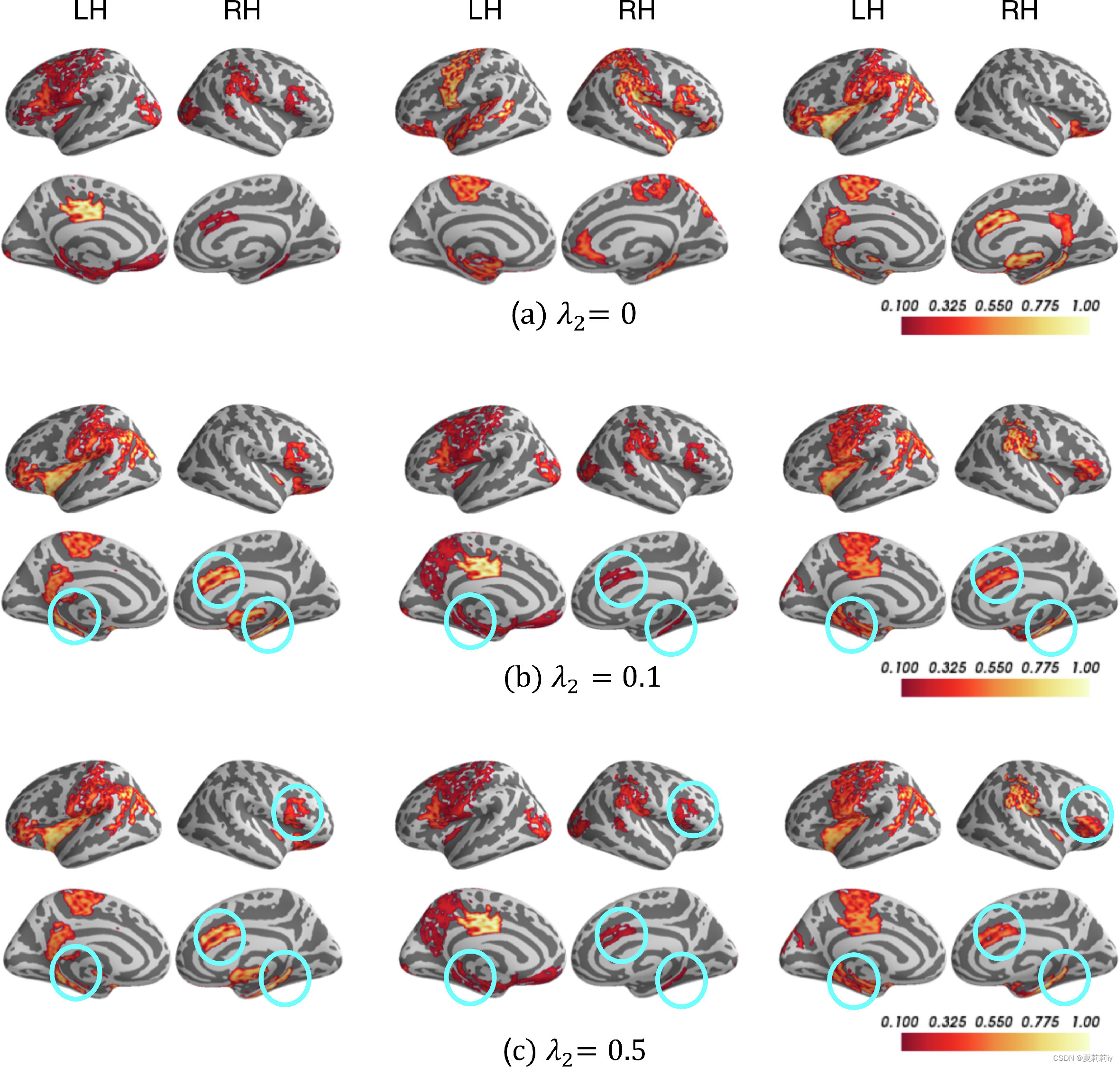
（3）Validating salient ROIs

①After twice 0.5 pooling, 84 ROIs are reduce to 21.

②In Biopoint, they chose putamen(壳核), thalamus(丘脑), temporal gyrus(颞回) and insular(岛叶), occipital lobe(枕叶) for HC, frontal gyrus(额回), temporal lobe(颞叶), cingulate gyrus(扣带回), occipital pole(枕极), and angular gyrus(角回) for ASD, Hippocampus(海马) and temporal polefor(颞极) all. （所以说为啥不都选一样的？）

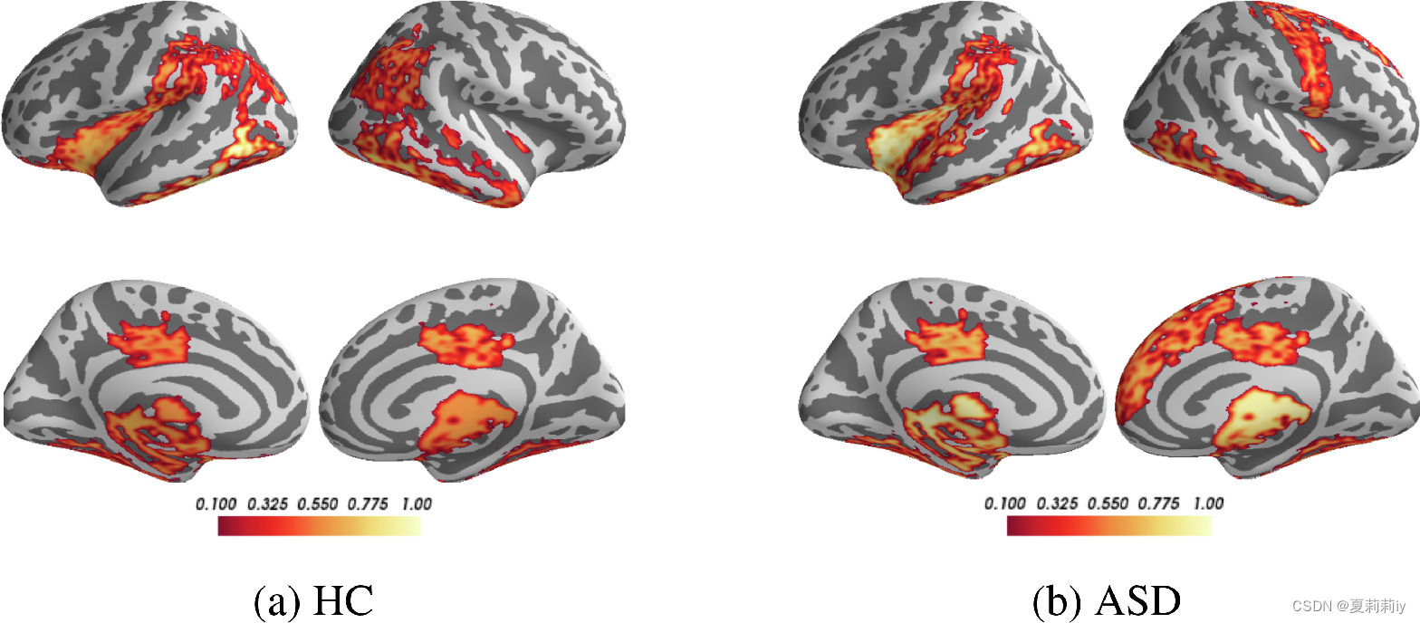
③In this picture, ASD is defective in social communication, perception and execution.

④They use afor fMRI data analysis platform Neurosynth and divide 7 tasks: gambling, language, motor, relational, social, working memory (WM) and emotion. Then get heatmanp with each element divided by the largest absolute value in its column.（哎我还是很疑惑为什么是二维还是同样的xy轴）

post-hoc adj.因果的

（4）Node clustering patterns in Ra-GConv layer

①Similar spatial pattern formed in Biopoint but not in HCP.

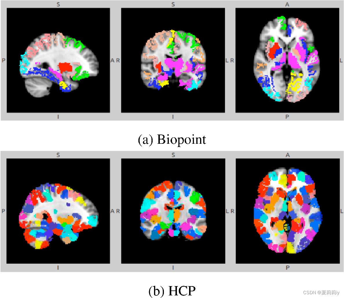
②The horizontal axis represents the number of ROIs, and the vertical axis represents the number of communities. This figure distinguishes the scores of $\alpha ^{+}$ under Biopoint and HCP.

corroborate vt.证实;确证(陈述、理论等)

2.4. Discussion

2.4.1. The model

（1）Innovation

①Setting different kernel for each community in Ra-GConv layers

②Novel regularization approach, unit loss, GLC loss and TPK loss

（2）Group-based analysis such as general linear model (GLM), principal component analysis (PCA) and independent component analysis (ICA) and individual-level analysis such as some deterministic models like connectome-based predictive modeling (CPM) can be used in fMRI analysis. Then, they affirmed the significance of parameter $\lambda _{2}$ in switching and comparing modes between individuals and groups.

2.4.2. Limitation and future work

（1）They reckon dynamical graph might be a improvement.

（2）For every data, they just try one graph. Ergo, multiple different graph might be a possible way.

（3）They think every parameter needs to be considered

（4）Considering integrate multi-modality data

2.5. Conclusions

Obviously, they conclude. And they say, em, the model is generalizable.

3. Reference List

Li, X. et al. (2021) 'BrainGNN: Interpretable Brain Graph Neural Network for fMRI Analysis', Medical Image Analysis, vol. 74, 102233. doi: Redirecting

Otsuzuki, T. et al. (2020) 'Regularized Pooling', Cornell University. doi: https://doi.org/10.48550/arXiv.2005.03709

这篇关于[论文精读]BrainGNN: Interpretable Brain Graph Neural Network for fMRI Analysis的文章就介绍到这儿，希望我们推荐的文章对编程师们有所帮助！