本文主要是介绍5、梯度下降法,牛顿法,高斯-牛顿迭代法,希望对大家解决编程问题提供一定的参考价值,需要的开发者们随着小编来一起学习吧!
1、梯度下降


2、牛顿法


3、高斯-牛顿迭代法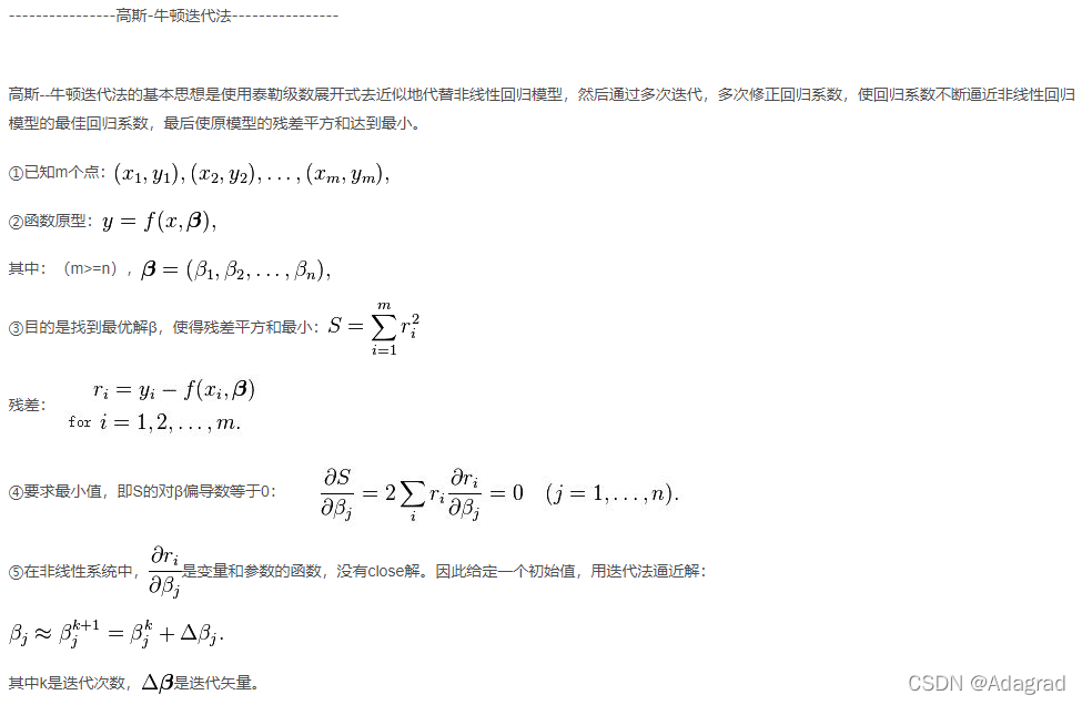


4、代码部分
1.梯度下降法代码
批量梯度下降法c++代码:
/*
需要参数为theta:theta0,theta1
目标函数:y=theta0*x0+theta1*x1;
*/
#include <iostream>
using namespace std;int main()
{float matrix[4][2] = { { 1, 1 }, { 2, 1 }, { 2, 2 }, { 3, 4 } };float result[4] = {5,6.99,12.02,18};float theta[2] = {0,0};float loss = 10.0;for (int i = 0; i < 10000 && loss>0.0000001; ++i){float ErrorSum = 0.0;float cost[2] = { 0.0, 0.0 };for (int j = 0; j <4; ++j){float h = 0.0;for (int k = 0; k < 2; ++k){h += matrix[j][k] * theta[k];}ErrorSum = result[j] - h;for (int k = 0; k < 2; ++k){cost[k] = ErrorSum*matrix[j][k];}}for (int k = 0; k < 2; ++k){theta[k] = theta[k] + 0.01*cost[k] / 4;}cout << "theta[0]=" << theta[0] << "\n" << "theta[1]=" << theta[1] << endl;loss = 0.0;for (int j = 0; j < 4; ++j){float h2 = 0.0;for (int k = 0; k < 2; ++k){h2 += matrix[j][k] * theta[k];}loss += (h2 - result[j])*(h2 - result[j]);}cout << "loss=" << loss << endl;}return 0;
}
2、随机梯度下降法C++代码:
/*
需要参数为theta:theta0,theta1
目标函数:y=theta0*x0+theta1*x1;
*/
#include <iostream>
using namespace std;int main()
{float matrix[4][2] = { { 1, 1 }, { 2, 1 }, { 2, 2 }, { 3, 4 } };float result[4] = {5,6.99,12.02,18};float theta[2] = {0,0};float loss = 10.0;for (int i = 0; i<1000 && loss>0.00001; ++i){float ErrorSum = 0.0;int j = i % 4;float h = 0.0;for (int k = 0; k<2; ++k){h += matrix[j][k] * theta[k];}ErrorSum = result[j] - h;for (int k = 0; k<2; ++k){theta[k] = theta[k] + 0.001*(ErrorSum)*matrix[j][k];}cout << "theta[0]=" << theta[0] << "\n" << "theta[1]=" << theta[1] << endl;loss = 0.0;for (int j = 0; j<4; ++j){float sum = 0.0;for (int k = 0; k<2; ++k){sum += matrix[j][k] * theta[k];}loss += (sum - result[j])*(sum - result[j]);}cout << "loss=" << loss << endl;}return 0;
}
3、牛顿法代码
实例,求解二元方程:
x*x-2*x-y+0.5=0; (1)
x*x+4*y*y-4=0; (2)
#include<iostream>
#include<cmath>
#define N 2                     // 非线性方程组中方程个数
#define Epsilon 0.0001          // 差向量1范数的上限
#define Max 1000            //最大迭代次数using namespace std;const int N2 = 2 * N;
void func_y(float xx[N], float yy[N]);					//计算向量函数的因变量向量yy[N]
void func_y_jacobian(float xx[N], float yy[N][N]);		// 计算雅克比矩阵yy[N][N]
void inv_jacobian(float yy[N][N], float inv[N][N]); //计算雅克比矩阵的逆矩阵inv
void NewtonFunc(float x0[N], float inv[N][N], float y0[N], float x1[N]);   //由近似解向量 x0 计算近似解向量 x1int main()
{float x0[N] = { 2.0, 0.5 }, y0[N], jacobian[N][N], invjacobian[N][N], x1[N], errornorm;//再次X0初始值满足方程1,不满足也可int i, j, iter = 0;cout << "初始近似解向量:" << endl;for (i = 0; i < N; i++){cout << x0[i] << " ";}cout << endl;cout << endl;while (iter<Max){iter = iter + 1;cout << "第 " << iter << " 次迭代" << endl;   func_y(x0, y0);                             //计算向量函数的因变量向量func_y_jacobian(x0, jacobian);              //计算雅克比矩阵inv_jacobian(jacobian, invjacobian);        //计算雅克比矩阵的逆矩阵NewtonFunc(x0, invjacobian, y0, x1);        //由近似解向量 x0 计算近似解向量 x1errornorm = 0;for (i = 0; i<N; i++)errornorm = errornorm + fabs(x1[i] - x0[i]);if (errornorm<Epsilon)break;for (i = 0; i<N; i++)x0[i] = x1[i];}return 0;
}void func_y(float xx[N], float yy[N])//求函数的因变量向量
{float x, y;int i;x = xx[0];y = xx[1];yy[0] = x*x-2*x-y+0.5;yy[1] = x*x+4*y*y-4;cout << "函数的因变量向量:" << endl;for (i = 0; i<N; i++)cout << yy[i] << "  ";cout << endl;
}void func_y_jacobian(float xx[N], float yy[N][N])	//计算函数雅克比的值
{float x, y;int i, j;x = xx[0];y = xx[1];//yy[][]分别对x,y求导,组成雅克比矩阵yy[0][0] = 2*x-2;yy[0][1] = -1;yy[1][0] = 2*x;yy[1][1] = 8*y;cout << "雅克比矩阵:" << endl;for (i = 0; i<N; i++){for (j = 0; j < N; j++){cout << yy[i][j] << " ";}cout << endl;}cout << endl;
}void inv_jacobian(float yy[N][N], float inv[N][N])//雅克比逆矩阵
{float aug[N][N2], L;int i, j, k;cout << "计算雅克比矩阵的逆矩阵:" << endl;for (i = 0; i<N; i++){for (j = 0; j < N; j++){aug[i][j] = yy[i][j];}for (j = N; j < N2; j++){if (j == i + N) aug[i][j] = 1;else  aug[i][j] = 0;}}for (i = 0; i<N; i++){for (j = 0; j < N2; j++){cout << aug[i][j] << " ";}cout << endl;}cout << endl;for (i = 0; i<N; i++){for (k = i + 1; k<N; k++){L = -aug[k][i] / aug[i][i];for (j = i; j < N2; j++){aug[k][j] = aug[k][j] + L*aug[i][j];}}}for (i = 0; i<N; i++){for (j = 0; j<N2; j++){cout << aug[i][j] << " ";}cout << endl;}cout << endl;for (i = N - 1; i>0; i--){for (k = i - 1; k >= 0; k--){L = -aug[k][i] / aug[i][i];for (j = N2 - 1; j >= 0; j--){aug[k][j] = aug[k][j] + L*aug[i][j];}}}for (i = 0; i<N; i++){for (j = 0; j < N2; j++){cout << aug[i][j] << " ";}cout << endl;}cout << endl;for (i = N - 1; i >= 0; i--){for (j = N2 - 1; j >= 0; j--){aug[i][j] = aug[i][j] / aug[i][i];}}for (i = 0; i<N; i++){for (j = 0; j < N2; j++){cout << aug[i][j] << " ";}cout << endl;for (j = N; j < N2; j++){inv[i][j - N] = aug[i][j];}}cout << endl;cout << "雅克比矩阵的逆矩阵: " << endl;for (i = 0; i<N; i++){for (j = 0; j < N; j++){cout << inv[i][j] << " ";}cout << endl;}cout << endl;
}void NewtonFunc(float x0[N], float inv[N][N], float y0[N], float x1[N])
{int i, j;float sum = 0;for (i = 0; i<N; i++){sum = 0;for (j = 0; j < N; j++){sum = sum + inv[i][j] * y0[j];}x1[i] = x0[i] - sum;}cout << "近似解向量:" << endl;for (i = 0; i < N; i++){cout << x1[i] << "  ";}cout << endl;
}
4、高斯-牛顿迭代法代码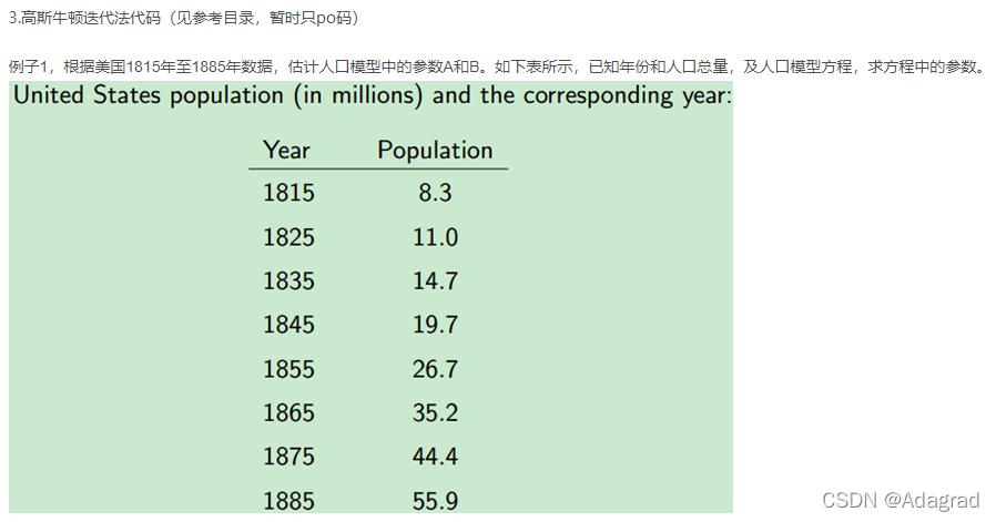
#include <cstdio>
#include <vector>
#include <opencv2/core/core.hpp>  using namespace std;
using namespace cv;const double DERIV_STEP = 1e-5;
const int MAX_ITER = 100;void GaussNewton(double(*Func)(const Mat &input, const Mat params), const Mat &inputs, const Mat &outputs, Mat params);double Deriv(double(*Func)(const Mat &input, const Mat params),const Mat &input, const Mat params, int n);// The user defines their function here
double Func(const Mat &input, const Mat params);int main()
{// For this demo we're going to try and fit to the function  // F = A*exp(t*B), There are 2 parameters: A B  int num_params = 2;// Generate random data using these parameters  int total_data = 8;Mat inputs(total_data, 1, CV_64F);Mat outputs(total_data, 1, CV_64F);//load observation data  for (int i = 0; i < total_data; i++) {inputs.at<double>(i, 0) = i + 1;  //load year  }//load America population  outputs.at<double>(0, 0) = 8.3;outputs.at<double>(1, 0) = 11.0;outputs.at<double>(2, 0) = 14.7;outputs.at<double>(3, 0) = 19.7;outputs.at<double>(4, 0) = 26.7;outputs.at<double>(5, 0) = 35.2;outputs.at<double>(6, 0) = 44.4;outputs.at<double>(7, 0) = 55.9;// Guess the parameters, it should be close to the true value, else it can fail for very sensitive functions!  Mat params(num_params, 1, CV_64F);//init guess  params.at<double>(0, 0) = 6;params.at<double>(1, 0) = 0.3;GaussNewton(Func, inputs, outputs, params);printf("Parameters from GaussNewton: %f %f\n", params.at<double>(0, 0), params.at<double>(1, 0));return 0;
}double Func(const Mat &input, const Mat params)
{// Assumes input is a single row matrix  // Assumes params is a column matrix  double A = params.at<double>(0, 0);double B = params.at<double>(1, 0);double x = input.at<double>(0, 0);return A*exp(x*B);
}//calc the n-th params' partial derivation , the params are our  final target
double Deriv(double(*Func)(const Mat &input, const Mat params), const Mat &input, const Mat params, int n)
{// Assumes input is a single row matrix  // Returns the derivative of the nth parameter  Mat params1 = params.clone();Mat params2 = params.clone();// Use central difference  to get derivative  params1.at<double>(n, 0) -= DERIV_STEP;params2.at<double>(n, 0) += DERIV_STEP;double p1 = Func(input, params1);double p2 = Func(input, params2);double d = (p2 - p1) / (2 * DERIV_STEP);return d;
}void GaussNewton(double(*Func)(const Mat &input, const Mat params),const Mat &inputs, const Mat &outputs, Mat params)
{int m = inputs.rows;int n = inputs.cols;int num_params = params.rows;Mat r(m, 1, CV_64F); // residual matrix  Mat Jf(m, num_params, CV_64F); // Jacobian of Func()  Mat input(1, n, CV_64F); // single row input  double last_mse = 0;for (int i = 0; i < MAX_ITER; i++) {double mse = 0;for (int j = 0; j < m; j++) {for (int k = 0; k < n; k++) {//copy Independent variable vector, the year  input.at<double>(0, k) = inputs.at<double>(j, k);}r.at<double>(j, 0) = outputs.at<double>(j, 0) - Func(input, params);//diff between estimate and observation population  mse += r.at<double>(j, 0)*r.at<double>(j, 0);for (int k = 0; k < num_params; k++) {Jf.at<double>(j, k) = Deriv(Func, input, params, k);}}mse /= m;// The difference in mse is very small, so quit  if (fabs(mse - last_mse) < 1e-8) {break;}Mat delta = ((Jf.t()*Jf)).inv() * Jf.t()*r;params += delta;//printf("%d: mse=%f\n", i, mse);  printf("%d %f\n", i, mse);last_mse = mse;}
}
#include <cstdio>
#include <vector>
#include <opencv2/core/core.hpp>  using namespace std;
using namespace cv;const double DERIV_STEP = 1e-5;
const int MAX_ITER = 100;void GaussNewton(double(*Func)(const Mat &input, const Mat params), const Mat &inputs, const Mat &outputs, Mat params);double Deriv(double(*Func)(const Mat &input, const Mat params),  const Mat &input, const Mat params, int n);double Func(const Mat &input, const Mat params);int main()
{// For this demo we're going to try and fit to the function  // F = A*sin(Bx) + C*cos(Dx),There are 4 parameters: A, B, C, D  int num_params = 4;// Generate random data using these parameters  int total_data = 100;double A = 5;double B = 1;double C = 10;double D = 2;Mat inputs(total_data, 1, CV_64F);Mat outputs(total_data, 1, CV_64F);for (int i = 0; i < total_data; i++) {double x = -10.0 + 20.0* rand() / (1.0 + RAND_MAX); // random between [-10 and 10]  double y = A*sin(B*x) + C*cos(D*x);// Add some noise  // y += -1.0 + 2.0*rand() / (1.0 + RAND_MAX);  inputs.at<double>(i, 0) = x;outputs.at<double>(i, 0) = y;}// Guess the parameters, it should be close to the true value, else it can fail for very sensitive functions!  Mat params(num_params, 1, CV_64F);params.at<double>(0, 0) = 1;params.at<double>(1, 0) = 1;params.at<double>(2, 0) = 8; // changing to 1 will cause it not to find the solution, too far away  params.at<double>(3, 0) = 1;GaussNewton(Func, inputs, outputs, params);printf("True parameters: %f %f %f %f\n", A, B, C, D);printf("Parameters from GaussNewton: %f %f %f %f\n", params.at<double>(0, 0), params.at<double>(1, 0),params.at<double>(2, 0), params.at<double>(3, 0));return 0;
}double Func(const Mat &input, const Mat params)
{// Assumes input is a single row matrix  // Assumes params is a column matrix  double A = params.at<double>(0, 0);double B = params.at<double>(1, 0);double C = params.at<double>(2, 0);double D = params.at<double>(3, 0);double x = input.at<double>(0, 0);return A*sin(B*x) + C*cos(D*x);
}double Deriv(double(*Func)(const Mat &input, const Mat params), const Mat &input, const Mat params, int n)
{// Assumes input is a single row matrix  // Returns the derivative of the nth parameter  Mat params1 = params.clone();Mat params2 = params.clone();// Use central difference  to get derivative  params1.at<double>(n, 0) -= DERIV_STEP;params2.at<double>(n, 0) += DERIV_STEP;double p1 = Func(input, params1);double p2 = Func(input, params2);double d = (p2 - p1) / (2 * DERIV_STEP);return d;
}void GaussNewton(double(*Func)(const Mat &input, const Mat params),const Mat &inputs, const Mat &outputs, Mat params)
{int m = inputs.rows;int n = inputs.cols;int num_params = params.rows;Mat r(m, 1, CV_64F); // residual matrix  Mat Jf(m, num_params, CV_64F); // Jacobian of Func()  Mat input(1, n, CV_64F); // single row input  double last_mse = 0;for (int i = 0; i < MAX_ITER; i++) {double mse = 0;for (int j = 0; j < m; j++) {for (int k = 0; k < n; k++) {input.at<double>(0, k) = inputs.at<double>(j, k);}r.at<double>(j, 0) = outputs.at<double>(j, 0) - Func(input, params);mse += r.at<double>(j, 0)*r.at<double>(j, 0);for (int k = 0; k < num_params; k++) {Jf.at<double>(j, k) = Deriv(Func, input, params, k);}}mse /= m;// The difference in mse is very small, so quit  if (fabs(mse - last_mse) < 1e-8) {break;}Mat delta = ((Jf.t()*Jf)).inv() * Jf.t()*r;params += delta; printf("%f\n", mse);last_mse = mse;}
}
梯度下降法,牛顿法,高斯-牛顿迭代法,附代码实现_Naruto_Q的博客-CSDN博客_梯度下降 高斯
这篇关于5、梯度下降法,牛顿法,高斯-牛顿迭代法的文章就介绍到这儿,希望我们推荐的文章对编程师们有所帮助!


