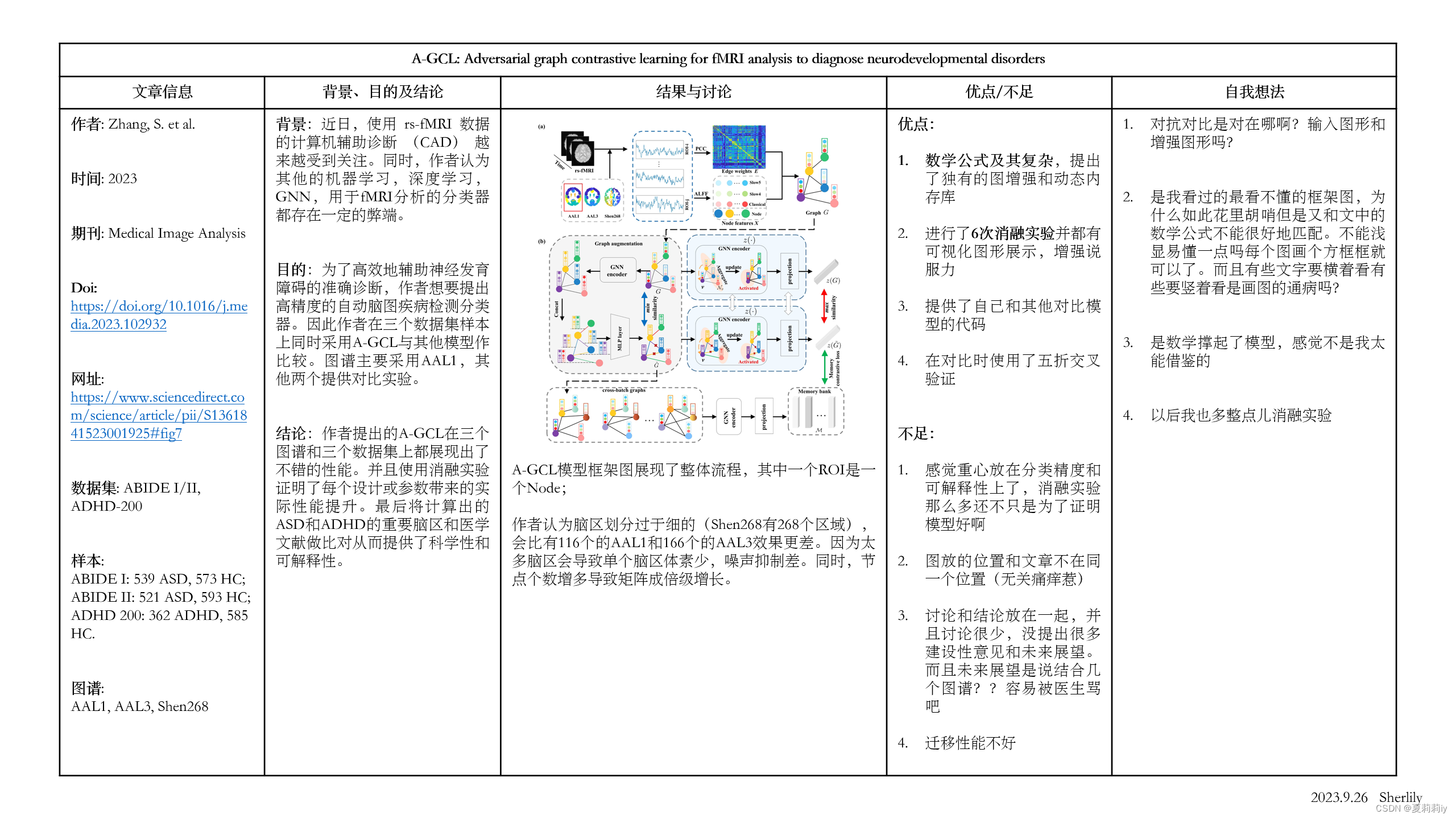
[论文精读]A-GCL: Adversarial graph contrastive learning for fMRI analysis to diagnose neurodevelopmental

本文主要是介绍[论文精读]A-GCL: Adversarial graph contrastive learning for fMRI analysis to diagnose neurodevelopmental，希望对大家解决编程问题提供一定的参考价值，需要的开发者们随着小编来一起学习吧！

论文全名：A-GCL: Adversarial graph contrastive learning for fMRI analysis to diagnose neurodevelopmental disorders

论文原文：A-GCL: Adversarial graph contrastive learning for fMRI analysis to diagnose neurodevelopmental disorders - ScienceDirect

论文代码：GitHub - qbmizsj/A-GCL: MedIA 2023

英文是纯手打的！论文原文的summarizing and paraphrasing。可能会出现难以避免的拼写错误和语法错误，若有发现欢迎评论指正！文章偏向于笔记，谨慎食用！

1. 省流版

1.1. 心得

1.2. 论文框架图

2. 原文逐段阅读

2.1. Abstract

2.2. Introduction

2.2.1. Related work

2.2.2. Contribution

2.3. Method

2.3.1. Graph construction

2.3.2. A-GCL

2.3.3. Classification and interpretation

2.3.4. Implementation details

2.4. Results

2.4.1. Experimental setup

2.4.2. Classification performance

2.4.4. Interpretation

2.5. Discussion and conclusion

2.5.1. Impact of atlas selection

2.5.2. Transfer learning between the two ABIDE datasets

2.5.3. Conclusion

3. Reference List

1. 省流版

1.1. 心得

（1）数学部分略显逆天

（2）整体框架图我是真的难评

（3）原文3.1.2给出了很多其他论文的代码

（4）曾在论文模型分类对比的时候怀疑过会不会是其他模型没训练好/参数没调合适，但是给自己模型调很好，但是被张老师以（如下图）驳回

（5）Fig2，3，4，5放的位置怎么回事

（6）有很多消融实验

（7）Discussion有点单薄啊，而且为什么discussion和conclusion放一起啊

（8）那你迁移学习不好不就代表泛化性差吗

（9）纯纯分类性能了

1.2. 论文框架图

2. 原文逐段阅读

2.1. Abstract

（1）Background: neurodevelopmental disorder diagnosis is limited to time consuming and biases from different examiners

（2）Model: they put forward adversarial self-supervised graph neural network based on graph contrastive learning (A-GCL)

（3）Data processing: fMRI, with feature classification.

（4）Node feature: 3 bands （波段） of the amplitude of low-frequency fluctuation (ALFF)

（5）Edge weight: average fMRI time series in different brain regions

（6）Contrastive learning: Bernoulli mask

（7）Dataset: ABIDE I, ABIDE II and ADHD-200

（8）Atlas: AAL1, AAL3, Shen268

2.2. Introduction

（1）Functional connectivity (FC) in resting-state functional Magnetic Resonance Imaging (rs-fMRI) mostly analysed by clinical experts themselves.

（2）In this paper, authors define normal controls as NC.

2.2.1. Related work

（1）Machine learning (ML) as SVM, MLP, RF, CNN, convolution-based autoencoder and deep learning (DL) as GNN made great progress in computer-aided diagnosis (CAD). （我想吐槽一下就是我在很多其他论文里面看到的都举的是很新的更针对脑科学的例子，这里全放这么早期又这么经典的...感觉略显敷衍...还是说这作者找不到那些代码来比对啊哈哈哈哈）

（2）⭐There are two categories of GNN, namely graph classification and node classification

（3）Graph classification: define a single brain as a graph. Such as BrainGB, BrainGNN, spatio-temporal attention GNN, node-edge graph attention network (NEGAT).

（4）Node classification: guess that each person constructs one graph. Such as: hierarchical graph convolutional network (GCN) etc.

（5）Graph contrastive learning (GCL): regard augmented version as positive sample which is close to original graph, put others as negative sample which are far away from original graph （什么玩意儿？）

（6）Limitations of GNN:

①Parameter update

②Adjacency matrix only ignores features of nodes

③Arbitrary truncation causes unsatisfactory creation of positive samples

canonical adj.典型的;经典的;(数学表达式)最简洁的;被收入真经篇目的;按照基督教会教规的

truncate vt.截断;截短，缩短，删节(尤指掐头或去尾) adj.截短的;被删节的

2.2.2. Contribution

（1）Adopt 3 bonds in ALFF from blood oxygen level-dependent (BOLD) signals

（2）A-GCL mainly foucs on edge-dropped version

（3）A-GCL do not drop any BOLD signal

（4）Build a dynamic memory bank which adopt queue structure to store samples from the same patch and different patch. This method save the memory of GPU and icrease the number of negative sample. All these are for the performance of model is highly rely on the number of negative sample.

（5）Conlusion of contributions

①Adversarial contrastive learning with a dynamic memory bank

②Multiple datasets and atlases（额，严格来说我觉得也不是特别大的贡献）

③Ablation study（其实我觉得这个严格来说也不算什么新的，但是作者在这好像提出了很多种消融实验啊。等我往后看看再说，是什么消融多样化吗）

④Explanation

（6）Information of graph and framework of A-GCL

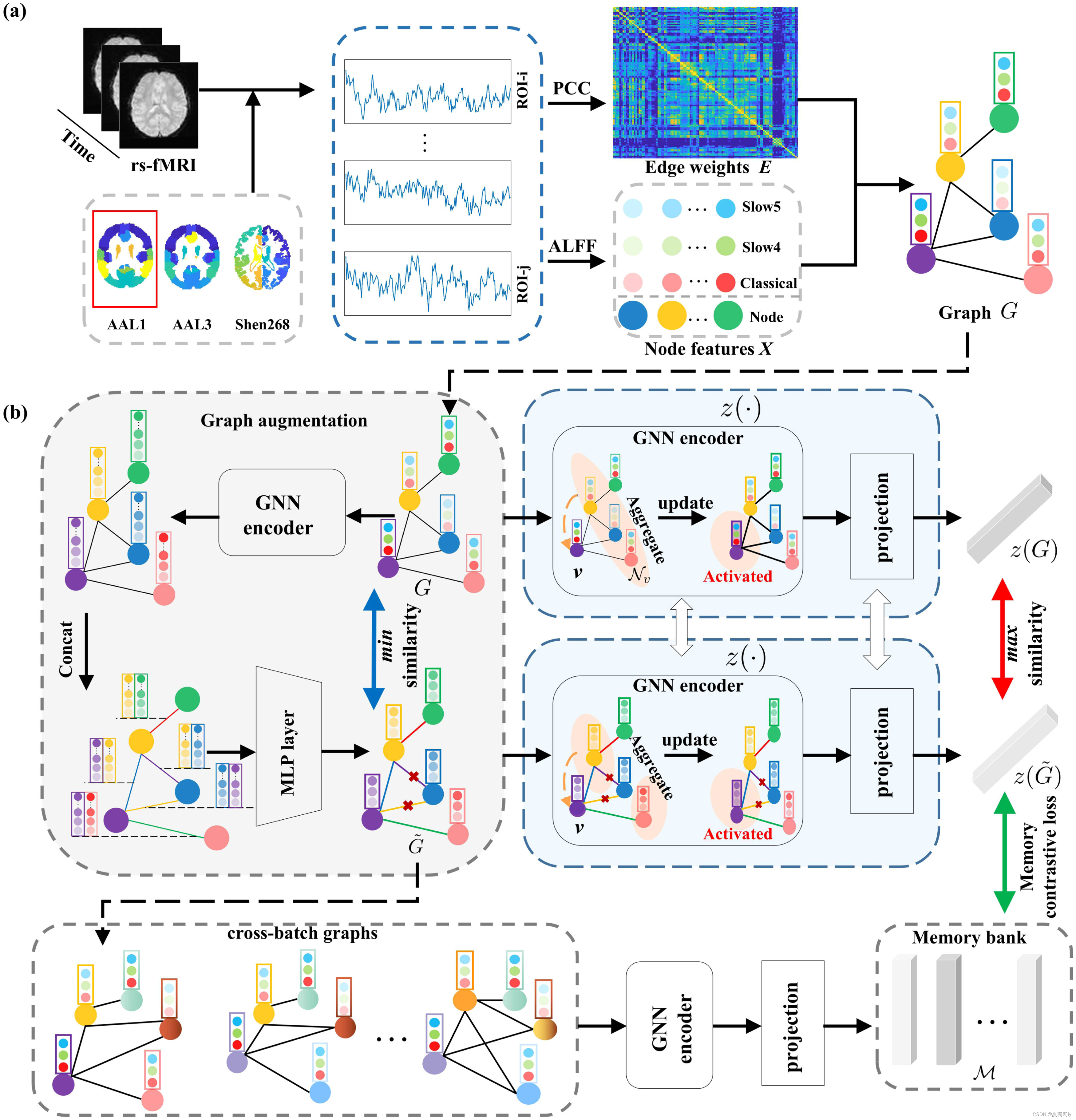
2.3. Method

2.3.1. Graph construction

（1）Authors set each ROI as a node, functional connectivity between ROI as an edge

（2）Mean time series: average of all BOLD signals in one region

（3）Edge weight: Pearson’s correlation coefficient (PCC) between mean time series in two regions

（4）Node feature: combine 3 ALFFs (Slow-5: 0.01–0.027 Hz, Slow-4: 0.027–0.073 Hz, classical: 0.01–0.08 Hz) in low-frequency range, then use Fourier transform of the mean time series

（5）Settings of graph

$G=(V,A,X,E)$

where $V=\{v:v=1,\ldots,M\}$ and $V$ denotes node set, $M$ denotes the number of ROIs;

$A=[a_{uw}:u,w\in V]\in\{0,1\}^{M\times M}$ , $A$ denotes adjacency matrix. All the existing edges are set by 1, otherwise 0;

$X=\left\{x_v\in\mathbb{R}^3:v\in V\right\}$ , $X$ denotes node features set;

$E=[e_{uw}\in\mathbb{R}:u,w\in V]\in\mathbb{R}^{M\times M}$ , $E$ denotes the edge weight matrix.

Besides, node features are normalized by:

$x_{v}=\frac{\bar{x}_{v}-min\, C}{max\, C-min\, C},\, then\, x_{v}\in \left [ 0,1 \right ]$

where $C$ denotes the channel value（这个我自己设的，我也不知道是什么啊）, $\bar{x}_{v}$ denotes original node feature;

The edge weights are normalized by:

$e_{uw}=\frac{\bar{e}_{uw}}{\left | max\, e \right |},\, then\, e_{uw}\in \left [ -1,1 \right ]$

where $\bar{e}$ denotes original edge weight.

2.3.2. A-GCL

（1）Graph augmentation

①Structure: graph isomorphism network (GIN) → feature concatenation → MLP

②GIN block

$h_v^{(k)}=g^{(k)}\left(h_v^{(k-1)},f^{(k)}\left(\left\{\left(h_u^{(k-1)},e_{uv}\right):u \in N_{v}\}\right\}\right)\right),k=1,2$

where $N_{v}$ denotes all the neighbor nodes of node $v$ ;

$h_{v}^{(0)}=x_{v}$ ;

$f^{(k)}$ is a funcion that adding features and edge weights together to a vector;

$g^{(k)}$ is MLP layer;

Therefore, the function can be rewritten as:

$h_{v}^{(k)}=MLP^{(k)}\left ( h_{v}^{(k-1)}+\sum_{u\in N_{v}}h_{u}^{(k-1)}e_{uv} \right )$

③Matrix form of GIN block

$\begin{aligned} &H^{\left(k-\frac12\right)}=\left(\mathbf{1}+A\circ E\right)H^{\left(k-1\right)},H^{\left(k\right)} \\ &=\mathrm{BN}\left(\sigma_{ReLU}\left(H^{\left(k-\frac12\right)}W_1^{(k)}+\mathbf{1}b_1^{(k)}\right)W_2^{(k)}+\mathbf{1}b_2^{(k)}\right) \end{aligned}$

where $H^{(k)}=\begin{pmatrix} h_{1}^{(k)}\\ h_{2}^{(k)}\\ ...\\ h_{M}^{(k)} \end{pmatrix}$ ;

$\circ$ denotes Hadamard product;

$\mathbf{1}$ denotes （？？？为什么说是M维全1的向量啊？？不应该是个矩阵吗）;

$W_1^{(k)}\in\mathbb{R}^{d^{(k-1)}\times d},b_1^{(k)}\in\mathbb{R}^{1\times d}\mathrm{~and~}W_2^{(k)}\in\mathbb{R}^{d\times d},b_2^{(k)}\in\mathbb{R}^{1\times d}, d^{(0)}=3,d^{(1)}=d$

are trainable parameters;

$BN$ denotes batch normalization;

④MLP layer

$\mu_{uv}=Sigmoid\left(ReLU\left(\tilde{x}_{uv}^\top W_3+b_3\right)W_4+b_4\right)$

where $W_3\in\mathbb{R}^{2d\times2d},b_3\in\mathbb{R}^{1\times2d},W_4\in\mathbb{R}^{2d\times1},b_4\in\mathbb{R}$ are trainable parameters;

$\tilde{x}_{v}=h_{v}^{(2)}$ , because there are two layers of GIN, $\tilde{x}_{v}$ reperesents the feature after learning;

Also, $\tilde{x}_{uv}=[\tilde{x}_{u};\tilde{x}_{v}]\in\mathbb{R}^{2d}$ denotes a combination of edge features.

④Dropout

$b_{uv}=Sigmoid\left(\left(\log\frac{\epsilon_{uv}}{1-\epsilon_{uv}}+\log\frac{\mu_{uv}}{1-\mu_{uv}}\right)/\tau\right)$

where $b_{uv}\sim\textit{Bernoulli }(\mu_{uv})$ , and drop any data if $b_{uv}=0$ ;

$\epsilon_{uv}\sim Uniform\left(0,1\right)$ ;

$\tau$ denotes a temperature parameter which controls the smoothness;

$\left(\log\frac{\epsilon_{uv}}{1-\epsilon_{uv}}+\log\frac{\mu_{uv}}{1-\mu_{uv}}\right)/\tau> 0$ when $\epsilon_{uv}\in \left ( 1-\mu _{uv},1 \right )$ ;

$\left(\log\frac{\epsilon_{uv}}{1-\epsilon_{uv}}+\log\frac{\mu_{uv}}{1-\mu_{uv}}\right)/\tau< 0$ when $\epsilon_{uv}\in \left ( 0,1-\mu _{uv} \right )$ .

⑤Summary of data augmentation

All in all, the process of augmentation can be written as $\tilde{G}=(V,A\circ B,X,E)$ ,

where $B\sim Bernoulli\left(\mu\left(G\right)\right)$

isomorphism n.同构；类质同象；类质同晶型（现象）；同（晶）型性

（2）Dynamic memory bank and loss function design

①Loss function 1 for bringing the same image feature closer and separating different image features

$I\left(z,\mu;\Re \right)=\frac{1}{\left|\Re \right|}\sum_{G\in\Re }\log\frac{\exp\left(sim\left(z(G),z\left(\tilde{G}\right)\right)\right)}{\sum_{G^{\prime}\in\Re \smallsetminus\{G\}}\exp\left(sim\left(z(G),z\left(\tilde{G}^{\prime}\right)\right)\right)}$

（什么是resp. $\tilde{G}^{\prime}$ ）

where $\Re$ is a batch of graph sets, $\left | \Re \right |$ is its cardinality（基数又是什么）.

②Similarity metric

$sim{(z_1,z_2)}=z_1^\top z_2/\left(\|z_1\|\|z_2\|\right)$

③Keep on droping out and minimize $R$ (?)

$R\left(\mu;\Re \right)=\frac{1}{\left|\Re \right|M^{2}}\sum_{G\in\Re }\mathbf{1}^{\top}\mu\left(G\right)\mathbf{1}$

④Loss function 2

$I\left(z,\mu;\Re ,\Im \right)=\frac{1}{\left|\Re \right|}\sum_{G\in\Re }\log\frac{\exp\left(sim\left(z(G),z\left(\widetilde{G}\right)\right)\right)}{\sum_{z^{\prime}\in\Im }\exp(sim(z(G),z^{\prime}))}$

where $\Im$ stores the previous batch of $z\left(\tilde{G}^{\prime}\right)$ in queue structure and is initialized by 0.

⑤Objeective function

$O=\min_{\mu}\max_{z}I\left(z,\mu;\Re \right)+\lambda_1R\left(\mu;\Re \right)+\lambda_2I\left(z,\mu;\Re ,\Im \right)$

where $\lambda _{1}$ and $\lambda _{2}$ are regularization coefficients;

and gradient descent/ascent bring $\mu$ and $z$ . (???????????)

2.3.3. Classification and interpretation

（1）Put SVM classifier in datasets:

（2）Interpretation

①Visualize the important connections in sparse graph

②Add all elements in one row in $A\circ B\circ E$ matrix as importance score. The score represents the degree of ROI connects

2.3.4. Implementation details

（1）Their experiment

①Framework: PyTorch

②Code: GitHub - qbmizsj/A-GCL: MedIA 2023GitHub - qbmizsj/A-GCL: MedIA 2023GitHub - qbmizsj/A-GCL: MedIA 2023

③Learning rate: 0.0005

④Embedded dimension $d$ : 32

⑤Batch size: 32

⑥The temperature $\tau$ : 1

⑦Regularization coefficient: $\lambda _{1}=2,\lambda _{2}=0.4$

⑧Length of $\Im$ : 256

（2）For new dataset

①Recommended batch size: 8 or 16 or 32 or 64

②Recommended learning rate :

$\mu\in \left \{ 0.0001, 0.0005, 0.001, 0.005, 0.01 \right \},z\in \left \{ 0.0005, 0.001, 0.01 \right \}$

2.4. Results

2.4.1. Experimental setup

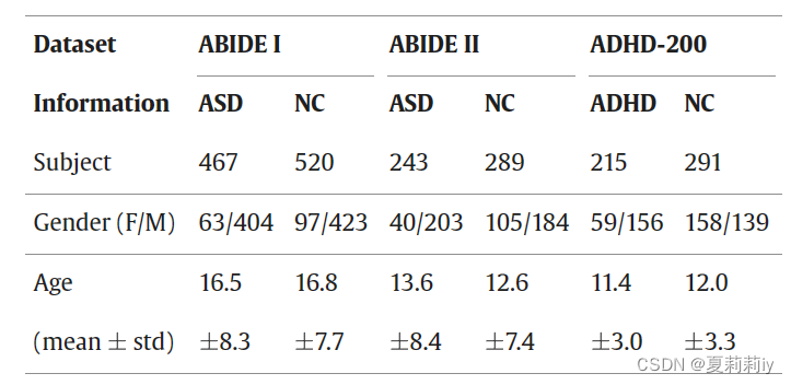
（1）Dataset and preprocessing

①fMRI processing pipeline: fMRIPrep

rs-fMRI reference image estimation, head-motion correction, slice timing correction, and susceptibility distortion correction are performed. For confounder removal, framewise displacement, global signals, and mean tissue signals are taken as the covariates and regressed out after registering the fMRI volumes to the standard MNI152 space.

②Define how they calculate time series, ALFF node features and FC matrix

③Setting 3 atlas, AAL1 with 116 regions, AAL3 with 166 regions, Shen268 with 268 regions

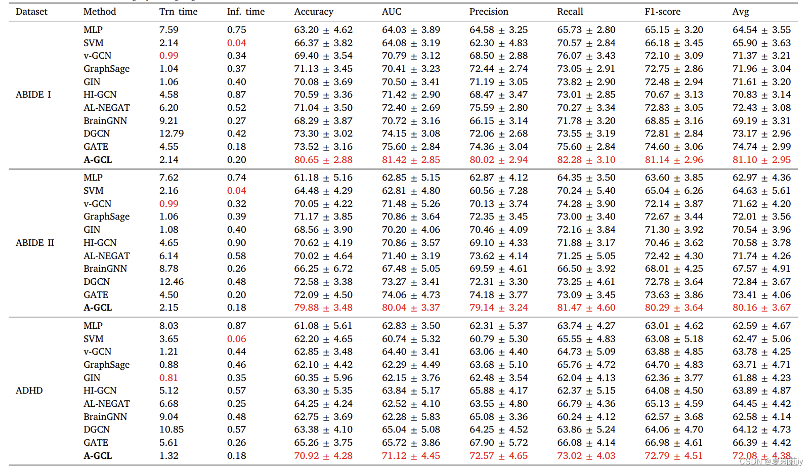
④Classification accuracy table in AAL1, while AAL3 and Shen268 are for examing the robustness in ablation study. Additionally, Trn time is training time and Inf. time is inference time

phenotypic adj.表（现）型的

confounder n.混淆;混杂因素;混杂变量;混杂因子;干扰因子

（2）Competing methods

①Provide the parameters setting in other models above

②⭐Provide codes of other models

（3）Evaluation strategy

①metrics: accuracy, sensitivity, specificity, F1-score, and AUC

②validation: 5 fold cross-validation

2.4.2. Classification performance

①Contrastive learning performs well in classification

②They compare data from 5-fold cross validation

（1）Transfer learning for ABIDE datasets

①Transfer learning on ABIDE I and ABIDE II

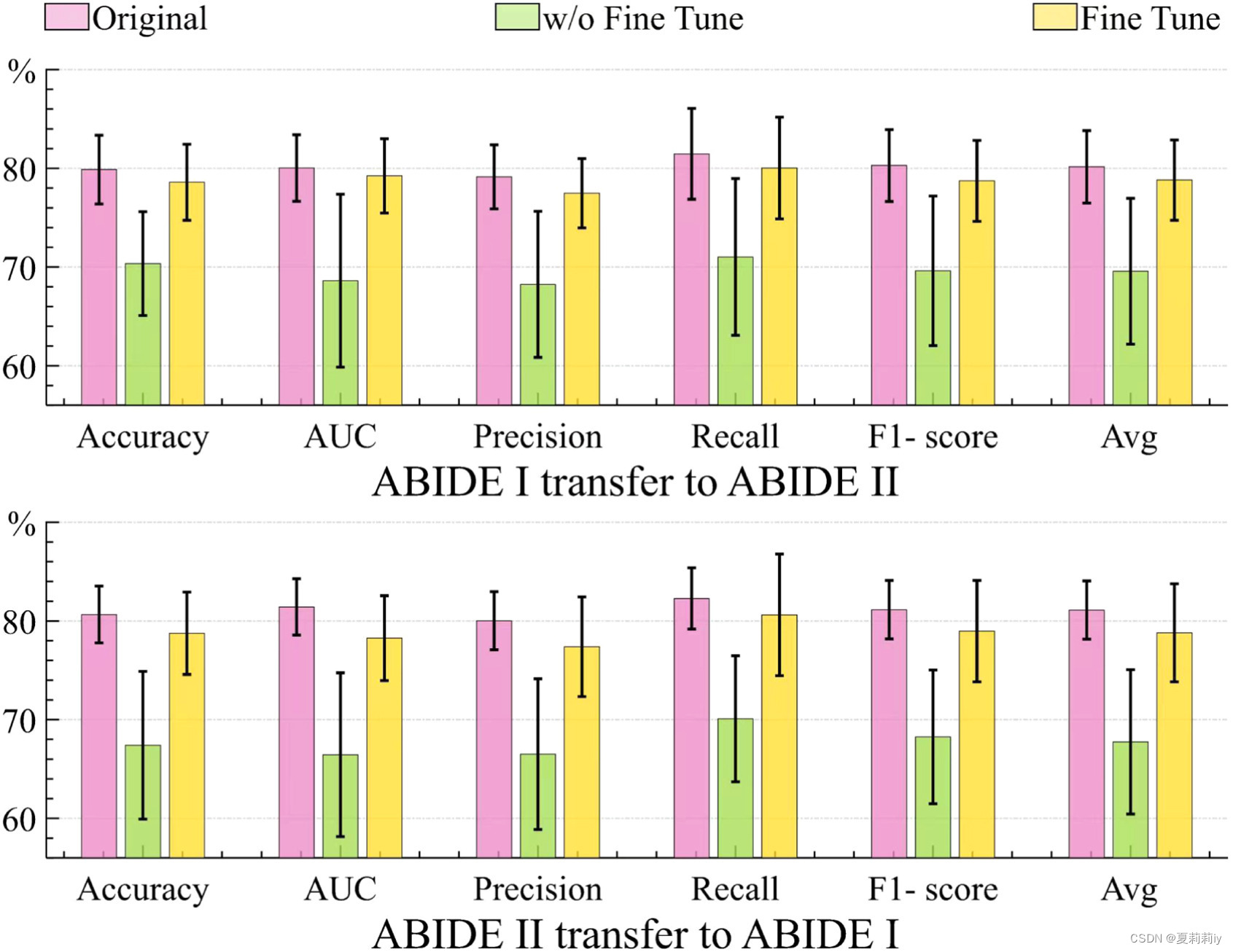
②The performance in transfer learning decrease 10% but still high

2.4.3. Ablation studies

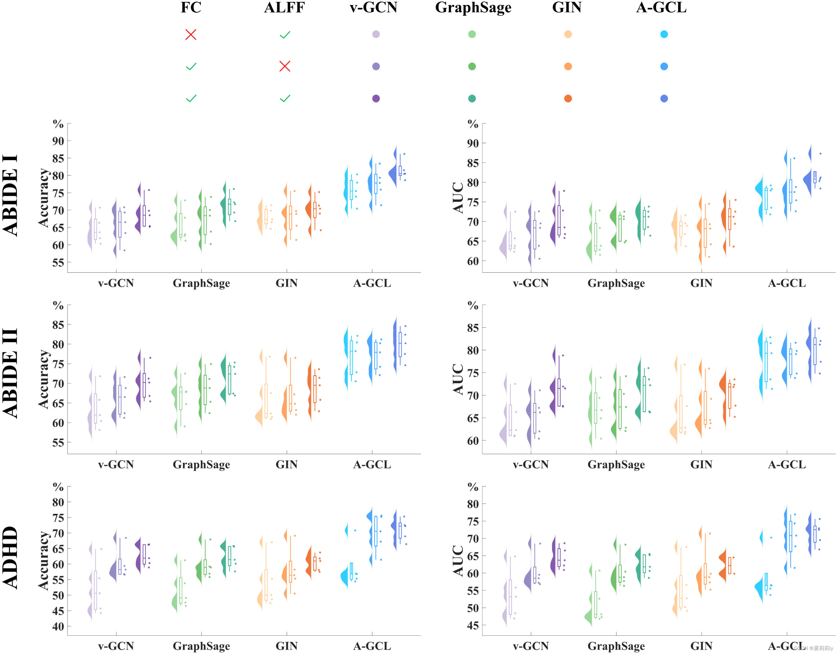
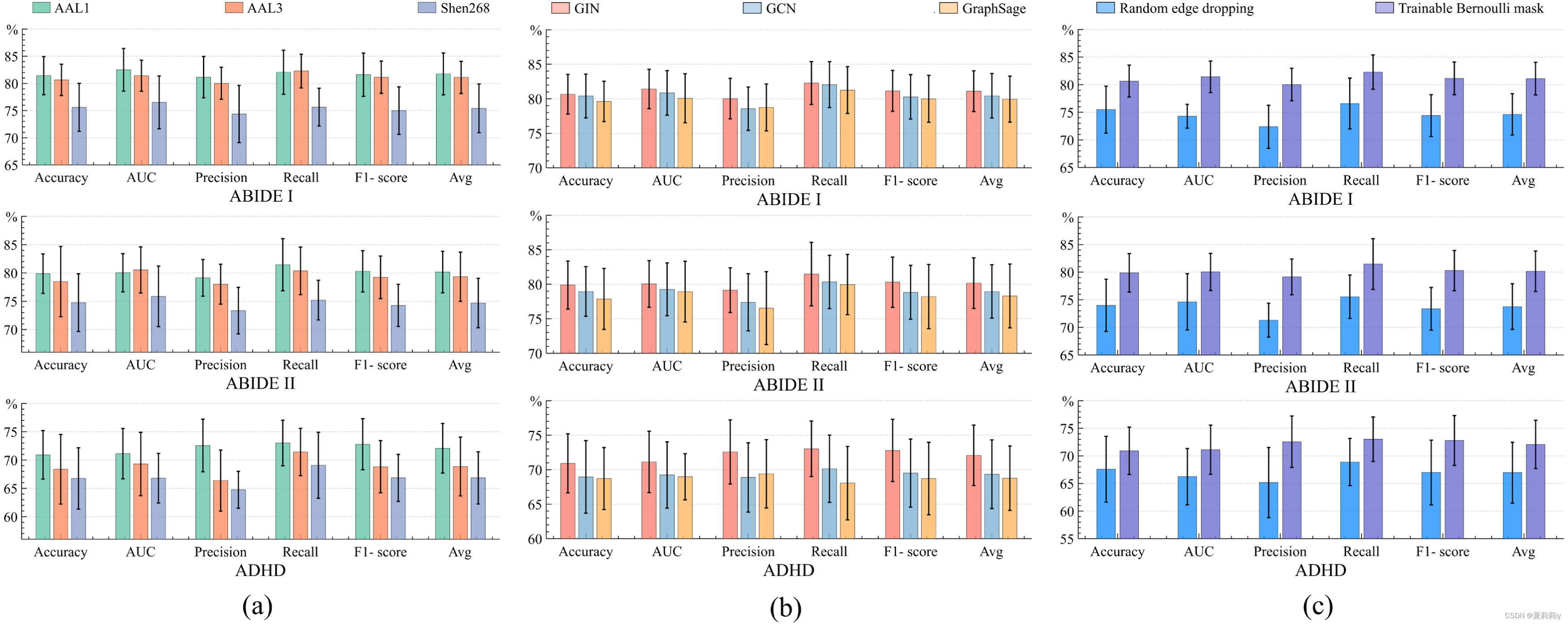
（1）Influence of different atlases on the three datasets

①Shen268 with more regions gets lower performance

②From 116 (AAL1) to 166 (AAL3) regions, ABIDE I is getting better but ABIDE II is not.

（2）Effectiveness of edge weights and node features

①Ablation study on how ALFF and FC influence the fMRI classification

where the first vertical line is setting all elements in FC matrix to 1, the second vertical line is setting all elements to 1 in ALFF feature vector.

（3）Influence of the GNN encoder

①Ablation study with a (a) atlases, (b) GNN encoders, and (c) edge-dropping strategies:

and presents robustness in different encoder.

（4）Influence of the graph augmentation strategy

①Normally the augmentation methods are random rotation, intensity scaling and random dropout

②The Bernoulli mask approach shows above (c) indicates its effectiveness

（5）Influence of the embedding dimension

①Ablation study on whether the embedding dimension will influence the classification performance, where the vertical lines are standard deviation:

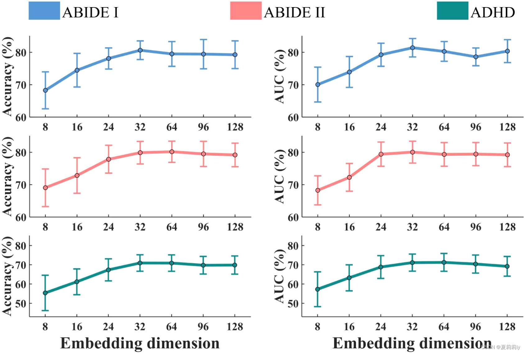
In this picture, authors reckon the more the dimension, the higher the accuracy and AUC value. However, they still guess 32 is the best dimension in that after that, the performance is getting steady but computing time increases sharply.

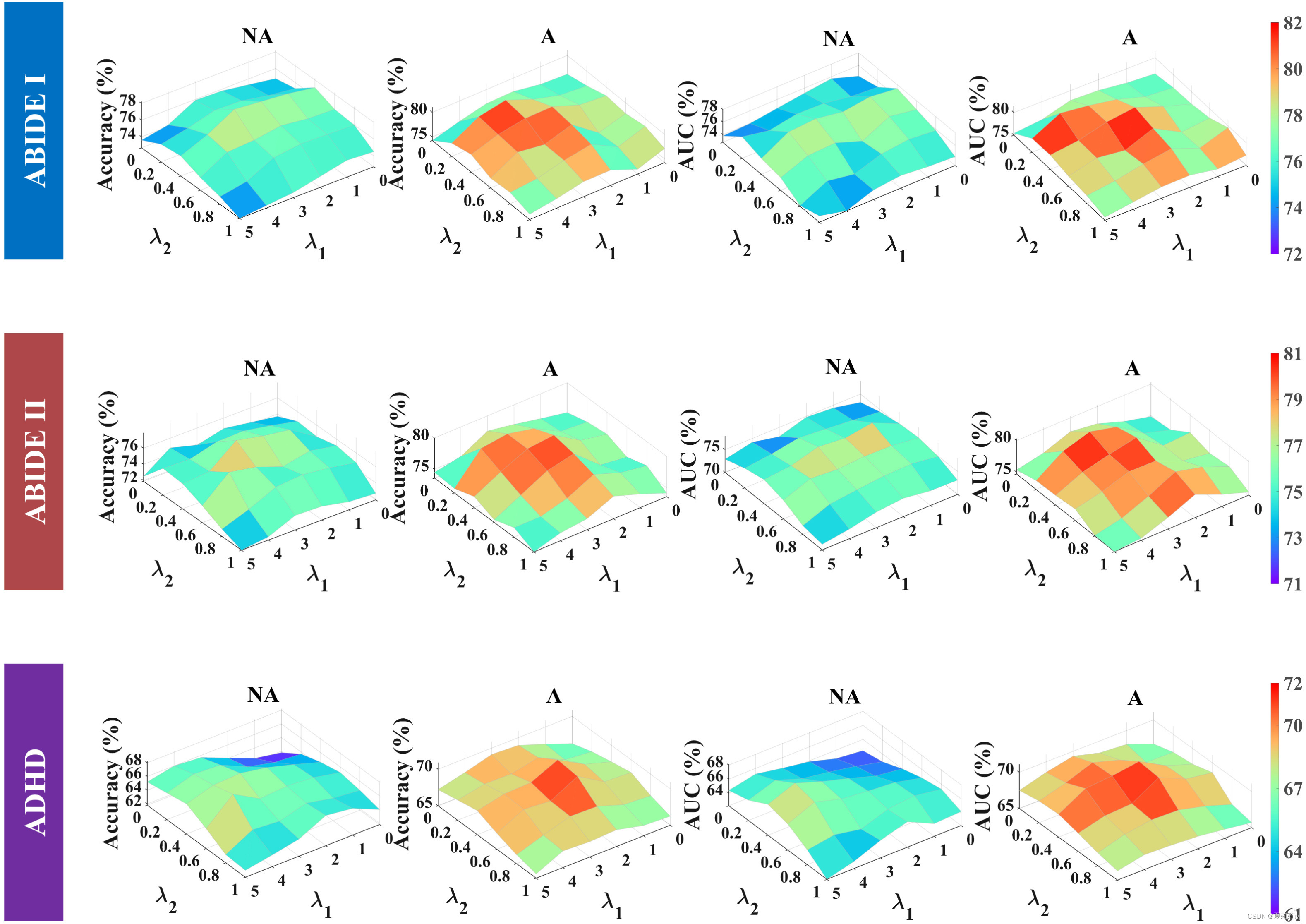
（6）Influence of λ1, λ2, and the max–min loss function

①The original adversarial loss function is:

$O=\min_{\mu}\max_{z}I\left(z,\mu;\Re \right)+\lambda_1R\left(\mu;\Re \right)+\lambda_2I\left(z,\mu;\Re ,\Im \right)$

However, for ablation study, authors change the function to

$O{}'=\min_{z,\mu}-I\left(z,\mu;\Re \right)+\lambda_1R\left(\mu;\Re \right)-\lambda_2I\left(z,\mu;\Re ,\Im \right)$

② How $\lambda _{1}$ and $\lambda _{2}$ works in AAL1, where A denotes adversarial, NA denotes non-adversarial

2.4.4. Interpretation

（1）Visualization of the learned Bernoulli mask

①Pictures of matrices and maps:

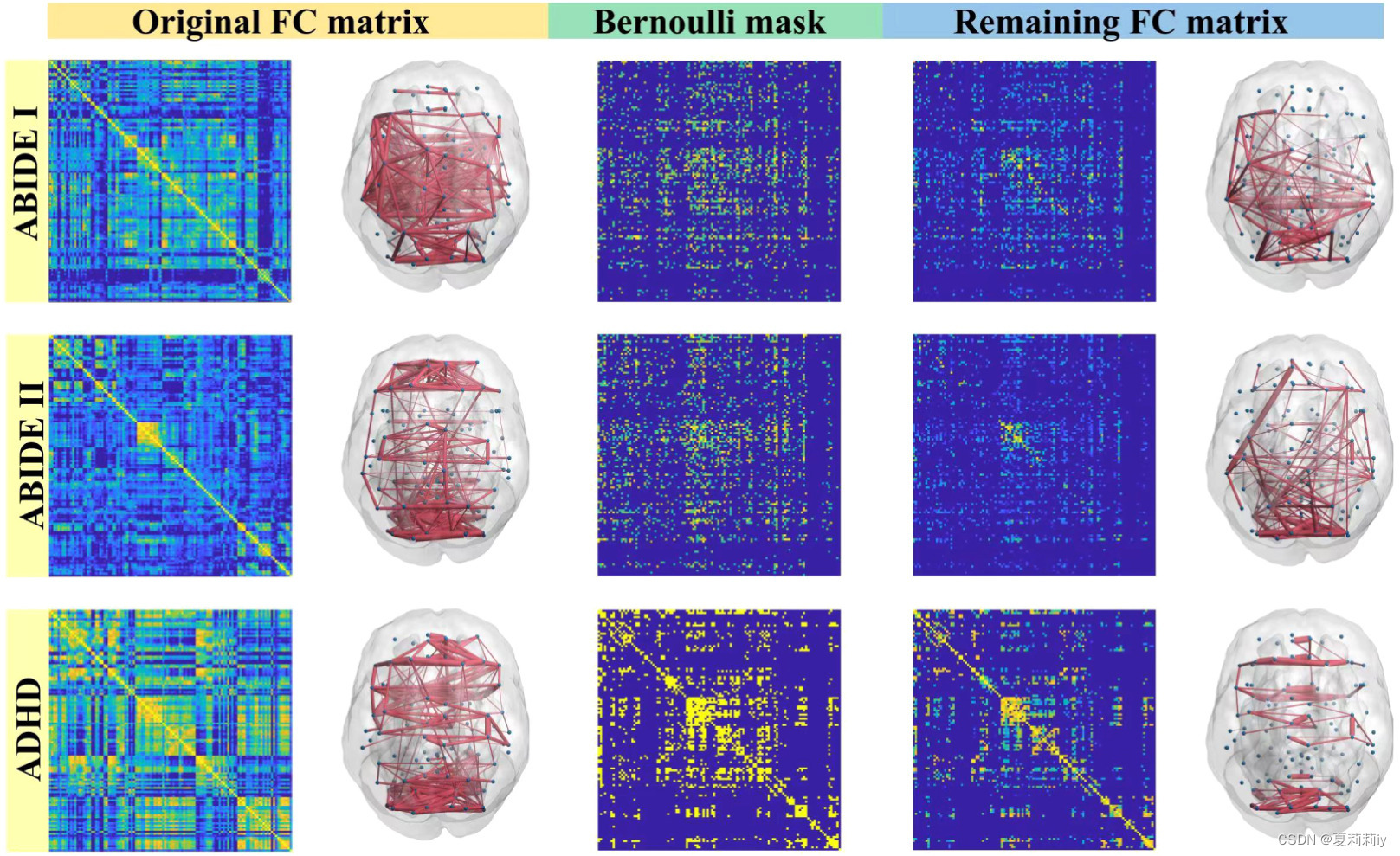
only the top 20% maps are shown above in that the whole FC maps are too dense.

②The correlation between two datasets are calculated by edge-dropped FC matrices/remaining FC matrices. Accordingly, the correlation coefficient between ABIDE I and ABIDE II is 0.8328, between ABIDE I/II and ADHD are 0.1422/0.1758.

（2）Visualization of the important brain regions

①Top 10 important regions

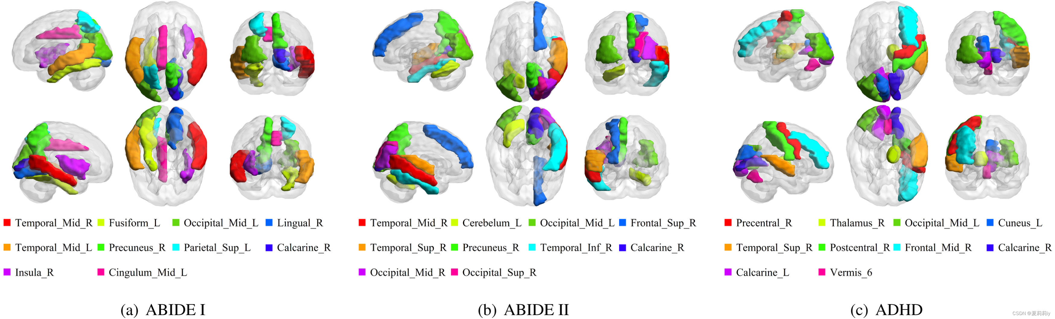
where they are calculated by the sum of FCs of a node in the edge-dropped graph, namely $\left ( A\circ B\circ E \right )\boldsymbol{1}$

2.5. Discussion and conclusion

2.5.1. Impact of atlas selection

（1）Authors speculate that more detailed partitioning in Shen268 results in a decrease in the average number of voxels that can be calculated. It also reduces noise suppression.

（2）On the other hand, there are more nodes in matrices which brings difficulty for calculating and optimization

（3）Authors suggest that reseachers can combine atlas to increase performance（这玩意儿真的能结合吗得看医生吧？）

2.5.2. Transfer learning between the two ABIDE datasets

Authors attribute the poor generalization ability to significant differences between the two datasets...

2.5.3. Conclusion

They combine different atlases, datasets, create A-GCL.

3. Reference List

Zhang, S. et al. (2023) 'A-GCL: Adversarial graph contrastive learning for fMRI analysis to diagnose neurodevelopmental disorders', Medical Image Analysis. vol. 90, 102932, doi: Redirecting

这篇关于[论文精读]A-GCL: Adversarial graph contrastive learning for fMRI analysis to diagnose neurodevelopmental的文章就介绍到这儿，希望我们推荐的文章对编程师们有所帮助！