本文主要是介绍R语言:microeco:一个用于微生物群落生态学数据挖掘的R包:第七:trans_network class,希望对大家解决编程问题提供一定的参考价值,需要的开发者们随着小编来一起学习吧!
# 网络是研究微生物生态共现模式的常用方法。在这一部分中,我们描述了trans_network类的所有核心内容。
# 网络构建方法可分为基于关联的和非基于关联的两种。有几种方法可以用来计算相关性和显著性。
#我们首先介绍了基于关联的网络。trans_network中的cal_cor参数用于选择相关计算方法。
> t1 <- trans_network$new(dataset = dataset, cal_cor = "base", taxa_level = "OTU", filter_thres = 0.0001, cor_method = "spearman")
> devtools::install_github('zdk123/SpiecEasi')
> library(SpiecEasi)
# SparCC method, require SpiecEasi package
> t1 <- trans_network$new(dataset = dataset, cal_cor = "SparCC", taxa_level = "OTU", filter_thres = 0.001, SparCC_simu_num = 100)
# require WGCNA package
> library(WGCNA)
> t1 <- trans_network$new(dataset = dataset, cal_cor = "WGCNA", taxa_level = "OTU", filter_thres = 0.0001, cor_method = "spearman")
#参数COR_cut可用于选择相关阈值。此外,COR_optimization = TRUE表示使用RMT理论寻找优化的相关阈值,而不是COR_cut。
> t1$cal_network(p_thres = 0.01, COR_optimization = TRUE)
# use arbitrary coefficient threshold to contruct network
> install.packages("rgexf")
> t1$save_network(filepath = "network.gexf")
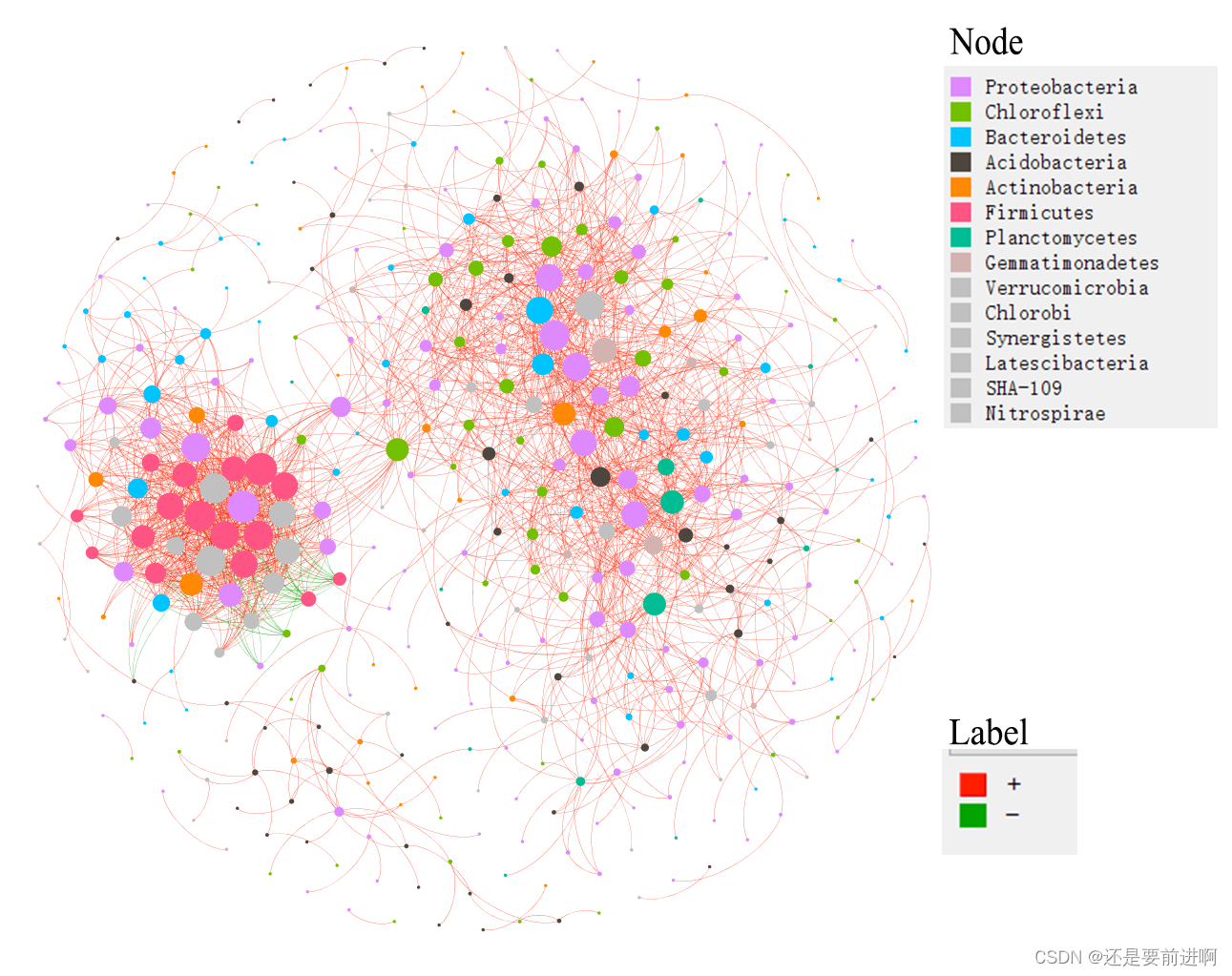
#根据Gephi中计算出的模块绘制网络并给出节点颜色。
#https://gephi.org/users/download/ 下载grephi

#现在,我们用门的信息显示节点的颜色,用正相关和负相关来显示边缘的颜色。所有使用的数据
#都存储在网络中。gexf文件,包括模块分类、门信息和边分类。
> t1$cal_network_attr()
Result is stored in object$res_network_attr ...
> t1$res_network_attrVertex                 4.070000e+02
Edge                   1.989000e+03
Average_degree         9.773956e+00
Average_path_length    2.784505e+00
Network_diameter       9.000000e+00
Clustering_coefficient 4.697649e-01
Density                2.407378e-02
Heterogeneity          1.193606e+00
Centralization         9.907893e-02
Modularity             5.485651e-01
> t1$cal_module()
Use cluster_fast_greedy function to partition modules ...
Totally, 25 modules are idenfified ...
Modules are assigned in network with attribute name -- module ...
> t1$get_node_table(node_roles = TRUE)
The nodes (22) with NaN in z will be filtered ...
Result is stored in object$res_node_table ...
> t1$plot_taxa_roles(use_type = 1)
Warning message:
Removed 22 rows containing missing values (`geom_point()`).
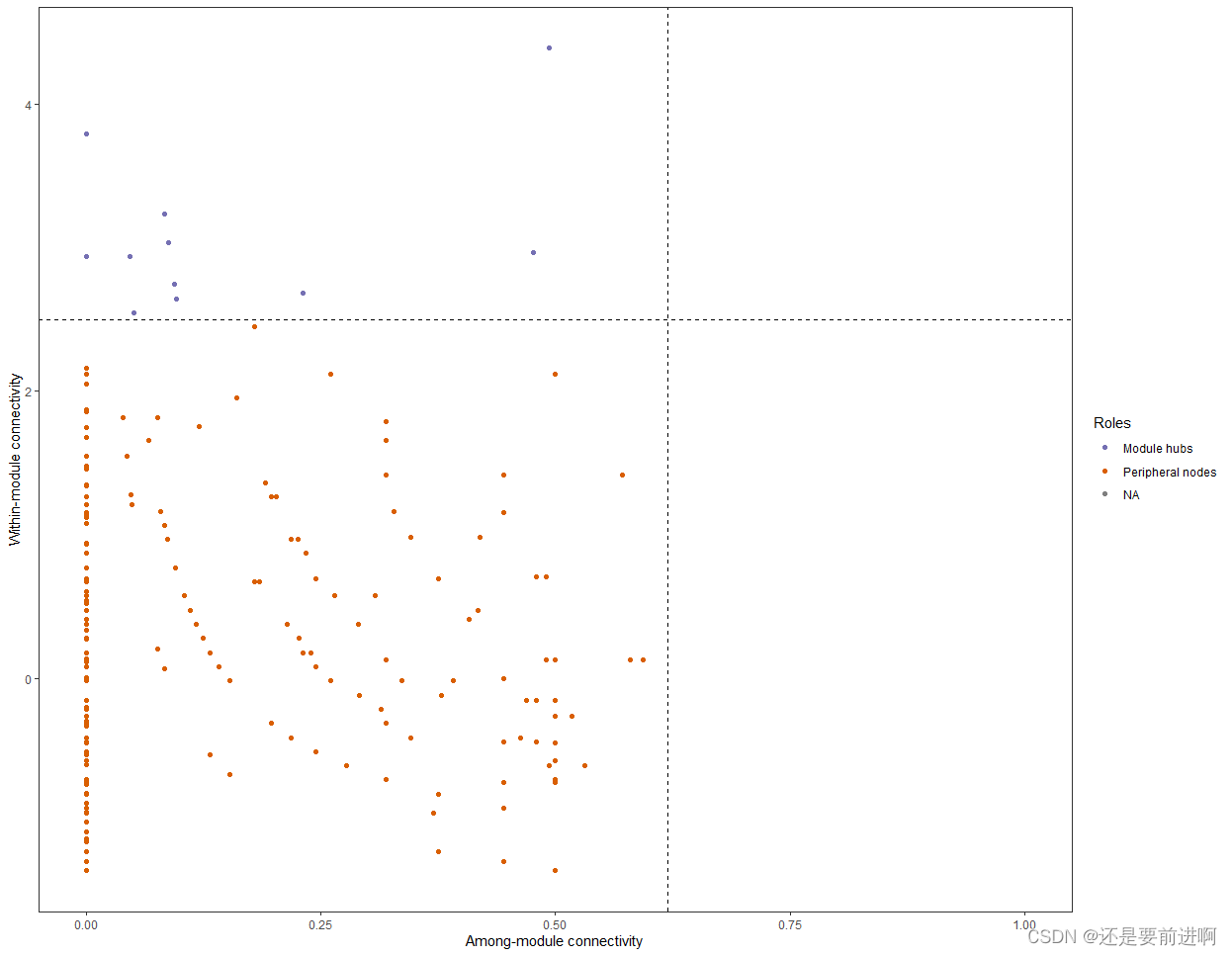
t1$plot_taxa_roles(use_type = 2)

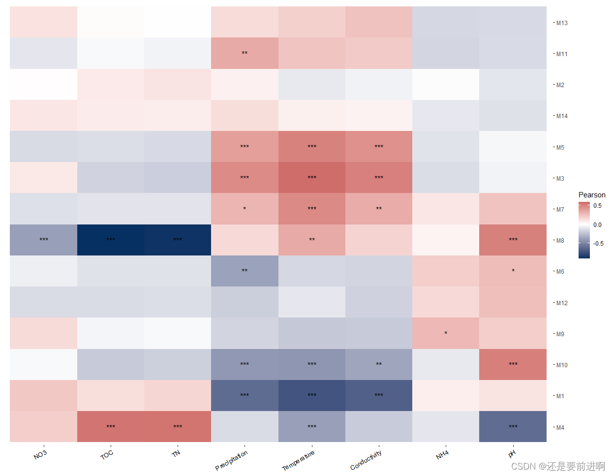
> t1$cal_eigen()
#然后用相关热图来显示特征基因与环境因素之间的关系。
> t2 <- trans_env$new(dataset = dataset, add_data = env_data_16S[, 4:11])
> t2$cal_cor(add_abund_table = t1$res_eigen)
> t2$plot_cor()
# 函数cal_sum_links()用于对从一个分类单元到另一个分类单元或同一分类单元中的链接(边)数求和。
# 函数plot_sum_links()用于显示函数cal_sum_links()的结果。这对于快速查看不同分类群之间或一个分类群内部连接了多少节点非常有用。
# 对于本教程中的“门”级别,函数cal_sum_links()将从一个门到另一个门或同一门中的连杆数求和。
# 所以圆形图外围的数字表示有多少条边或连接与门有关。例如,就Proteobacteria而言,
# 大约总共有900条边与Proteobacteria中的OTUs相关,其中大约有200条边将Proteobacteria中的两个OTUs连接起来,
# 大约有150条边将Proteobacteria中的OTUs与来自Chloroflexi的OTUs连接起来。
# calculate the links between or within taxonomic ranks
> t1$cal_sum_links(taxa_level = "Phylum")
# return t1$res_sum_links_pos and t1$res_sum_links_neg
# require chorddiag package
> devtools::install_github("mattflor/chorddiag", build_vignettes = TRUE)
> t1$plot_sum_links(plot_pos = TRUE, plot_num = 10)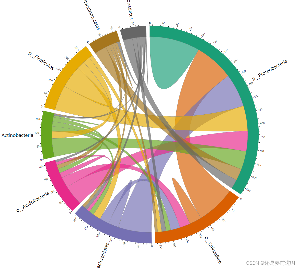
> #subset_network()函数可用于从网络中提取部分节点和这些节点之间的边。在这个函数中,应该使用node参数提供所需的节点。
> t1$subset_network(node = t1$res_node_type %>% .[.$module == "M1", ] %>% rownames, rm_single = TRUE)
IGRAPH 7df7c55 UNW- 407 1989 --
+ attr: name (v/c), taxa (v/c), Phylum (v/c), RelativeAbundance (v/n), module (v/c), label (e/c), weight (e/n)
+ edges from 7df7c55 (vertex names):[1] OTU_50   --OTU_357   OTU_50   --OTU_154   OTU_305  --OTU_3303  OTU_305  --OTU_2564  OTU_305  --OTU_30    OTU_1    --OTU_13824 OTU_1    --OTU_4731 [8] OTU_1    --OTU_34    OTU_1    --OTU_301   OTU_1    --OTU_668   OTU_1    --OTU_1169  OTU_1    --OTU_847   OTU_1    --OTU_1243  OTU_1    --OTU_266
[15] OTU_1    --OTU_1897  OTU_1    --OTU_1185  OTU_1    --OTU_1892  OTU_1    --OTU_1811  OTU_1    --OTU_126   OTU_1    --OTU_902   OTU_1    --OTU_351
[22] OTU_1    --OTU_264   OTU_1    --OTU_1173  OTU_1    --OTU_1866  OTU_1    --OTU_1848  OTU_1    --OTU_1204  OTU_41   --OTU_117   OTU_59   --OTU_78
[29] OTU_59   --OTU_357   OTU_59   --OTU_943   OTU_2733 --OTU_2725  OTU_4050 --OTU_7205  OTU_4050 --OTU_3522  OTU_4147 --OTU_1646  OTU_4147 --OTU_109
[36] OTU_4147 --OTU_7557  OTU_4147 --OTU_265   OTU_4147 --OTU_3164  OTU_4147 --OTU_8029  OTU_4147 --OTU_107   OTU_4147 --OTU_7648  OTU_4147 --OTU_3138
[43] OTU_4147 --OTU_1812  OTU_4147 --OTU_2784  OTU_4147 --OTU_426   OTU_4147 --OTU_1850  OTU_4147 --OTU_3712  OTU_4147 --OTU_3321  OTU_4147 --OTU_12327
[50] OTU_4147 --OTU_3159  OTU_4147 --OTU_7630  OTU_4147 --OTU_1885  OTU_4147 --OTU_1827  OTU_4147 --OTU_7346  OTU_4147 --OTU_4531  OTU_4147 --OTU_1810
+ ... omitted several edges
> #然后,我们展示了下一个实现的网络构建方法:SpiecEasi R包中的SpiecEasi(稀疏逆协方差估计for Ecological Association Inference)网络。
> # cal_cor select NA
> t1 <- trans_network$new(dataset = dataset, cal_cor = NA, taxa_level = "OTU", filter_thres = 0.0005)
After filtering, 301 features are remained ...
> # require SpiecEasi package  https://github.com/zdk123/SpiecEasi
> t1$cal_network(network_method = "SpiecEasi")
---------------- 2024-03-18 15:42:16.310147 : Start ----------------
Applying data transformations...
Selecting model with pulsar using stars...
Fitting final estimate with mb...
done
---------------- 2024-03-18 15:48:05.015648 : Finish ----------------
The result network is stored in object$res_network ...
> t1$res_network
IGRAPH da9387f UNW- 301 1595 --
+ attr: name (v/c), taxa (v/c), Phylum (v/c), RelativeAbundance (v/n), weight (e/n), label (e/c)
+ edges from da9387f (vertex names):[1] OTU_32  --OTU_238  OTU_32  --OTU_115  OTU_32  --OTU_578  OTU_32  --OTU_260  OTU_32  --OTU_62   OTU_32  --OTU_1283 OTU_32  --OTU_205  OTU_32  --OTU_315 [9] OTU_32  --OTU_64   OTU_32  --OTU_348  OTU_32  --OTU_345  OTU_32  --OTU_201  OTU_50  --OTU_408  OTU_50  --OTU_59   OTU_50  --OTU_3303 OTU_50  --OTU_117
[17] OTU_50  --OTU_318  OTU_50  --OTU_632  OTU_50  --OTU_67   OTU_50  --OTU_3052 OTU_50  --OTU_357  OTU_50  --OTU_771  OTU_50  --OTU_30   OTU_50  --OTU_674
[25] OTU_305 --OTU_59   OTU_305 --OTU_37   OTU_305 --OTU_3303 OTU_305 --OTU_146  OTU_305 --OTU_67   OTU_305 --OTU_578  OTU_305 --OTU_3052 OTU_305 --OTU_28
[33] OTU_305 --OTU_30   OTU_305 --OTU_26   OTU_305 --OTU_92   OTU_305 --OTU_58   OTU_408 --OTU_23   OTU_408 --OTU_22   OTU_408 --OTU_117  OTU_408 --OTU_169
[41] OTU_408 --OTU_27   OTU_408 --OTU_217  OTU_408 --OTU_3052 OTU_408 --OTU_1830 OTU_408 --OTU_530  OTU_6426--OTU_31   OTU_6426--OTU_515  OTU_6426--OTU_372
[49] OTU_6426--OTU_409  OTU_6426--OTU_293  OTU_6426--OTU_341  OTU_6426--OTU_1819 OTU_6426--OTU_1922 OTU_6426--OTU_970  OTU_6426--OTU_430  OTU_75  --OTU_31
[57] OTU_75  --OTU_22   OTU_75  --OTU_515  OTU_75  --OTU_204  OTU_75  --OTU_656  OTU_75  --OTU_839  OTU_75  --OTU_1922 OTU_75  --OTU_21   OTU_75  --OTU_431
+ ... omitted several edges
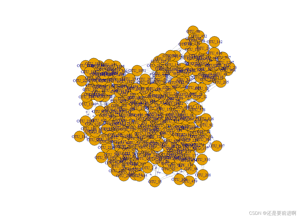
> t1$plot_network()
这一期跑了很久。大家慎跑。
这篇关于R语言:microeco:一个用于微生物群落生态学数据挖掘的R包:第七:trans_network class的文章就介绍到这儿,希望我们推荐的文章对编程师们有所帮助!


