本文主要是介绍深度学习模型部署(三)Onnxruntime部署yolov5实战,希望对大家解决编程问题提供一定的参考价值,需要的开发者们随着小编来一起学习吧!
模型分析
先使用yolov5下的yolo.py输出查看一下yolov5s的结构
python ./yolov5/models/yolo.py
YOLOv5 🚀 v7.0-287-g574331f9 Python-3.8.18 torch-2.2.1+cu118 CUDA:0 (NVIDIA GeForce RTX 3060 Laptop GPU, 6144MiB)
## 这里面的from是指输入来自哪一层,-1表示来自上一层,6表示来自第6层from  n    params  module                                  arguments                     0                -1  1      3520  models.common.Conv                      [3, 32, 6, 2, 2]              1                -1  1     18560  models.common.Conv                      [32, 64, 3, 2]                2                -1  1     18816  models.common.C3                        [64, 64, 1]                   3                -1  1     73984  models.common.Conv                      [64, 128, 3, 2]               4                -1  2    115712  models.common.C3                        [128, 128, 2]                 5                -1  1    295424  models.common.Conv                      [128, 256, 3, 2]              6                -1  3    625152  models.common.C3                        [256, 256, 3]                 7                -1  1   1180672  models.common.Conv                      [256, 512, 3, 2]              8                -1  1   1182720  models.common.C3                        [512, 512, 1]                 9                -1  1    656896  models.common.SPPF                      [512, 512, 5]                 10                -1  1    131584  models.common.Conv                      [512, 256, 1, 1]              11                -1  1         0  torch.nn.modules.upsampling.Upsample    [None, 2, 'nearest']          12           [-1, 6]  1         0  models.common.Concat                    [1]                           13                -1  1    361984  models.common.C3                        [512, 256, 1, False]          14                -1  1     33024  models.common.Conv                      [256, 128, 1, 1]              15                -1  1         0  torch.nn.modules.upsampling.Upsample    [None, 2, 'nearest']          16           [-1, 4]  1         0  models.common.Concat                    [1]                           17                -1  1     90880  models.common.C3                        [256, 128, 1, False]          18                -1  1    147712  models.common.Conv                      [128, 128, 3, 2]              19          [-1, 14]  1         0  models.common.Concat                    [1]                           20                -1  1    296448  models.common.C3                        [256, 256, 1, False]          21                -1  1    590336  models.common.Conv                      [256, 256, 3, 2]              22          [-1, 10]  1         0  models.common.Concat                    [1]                           23                -1  1   1182720  models.common.C3                        [512, 512, 1, False]          24      [17, 20, 23]  1    229245  Detect                                  [80, [[10, 13, 16, 30, 33, 23], [30, 61, 62, 45, 59, 119], [116, 90, 156, 198, 373, 326]], [128, 256, 512]]
YOLOv5s summary: 214 layers, 7235389 parameters, 7235389 gradients, 16.6 GFLOPsFusing layers...
YOLOv5s summary: 157 layers, 7225885 parameters, 7225885 gradients, 16.4 GFLOPs
可以看到yolov5s一共214层,层融合后还有157层
其中的C3层的结构是:
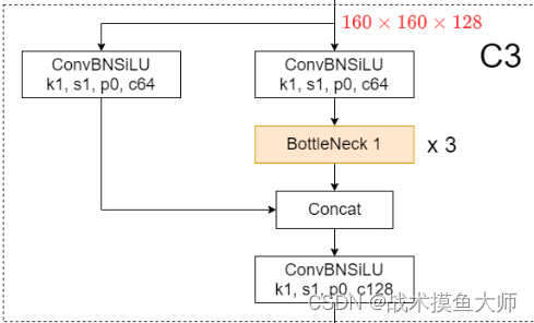

这里面的ConvBNSiLU就是指Conv+BN+SiLU,SiLU是ReLU的改进版激活函数,可以简单理解为y=x*sigmoid(x)。
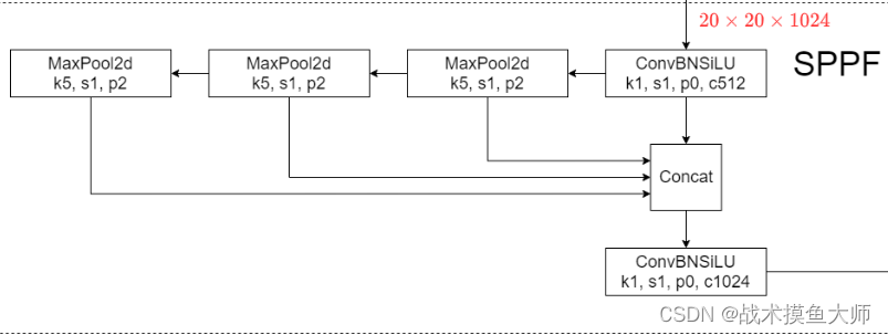
SPPF的结构如下,SPPF的作用是图像金字塔池化,进行多尺度特征融合:
目标检测的三件套:Backbone,Neck,Head,
yolov5的Backbone就是CSP-DarkNet53
Neck是PANet
head比较简单,就是三个尺度各一个Conv卷积层
(这是6.0版本的图,我们用的是7.0版本的模型,将就着看,反正大致结构差不多)

不过这些对于我们部署来说不重要,我们只需要看数据流以及模型的计算图就行,至于哪一部分叫什么名字无所谓,不care。
另外还可以看一下fusing layers到底fuse了哪些层
def fuse(self):"""Fuses Conv2d() and BatchNorm2d() layers in the model to improve inference speed."""LOGGER.info("Fusing layers... ")for m in self.model.modules():if isinstance(m, (Conv, DWConv)) and hasattr(m, "bn"):m.conv = fuse_conv_and_bn(m.conv, m.bn) # update convdelattr(m, "bn") # remove batchnormm.forward = m.forward_fuse # update forwardself.info()return self
我们可以看到,yolov5是将卷积和BN层融合到了一起
DWConv是指深度卷积depth-wise conv,相较于传统卷积的区别是一个输入channel卷积后对应一个输出channel,而不是多个输入channel卷积加和到一起对应一个输出channel,减少了计算量和参数量
具体fuse的代码如下,跟我们前面常见算子融合blog中讲的原理一模一样,不过并没有用torch自带的方法,而是自己实现的方法:
def fuse_conv_and_bn(conv, bn):"""Fuses Conv2d and BatchNorm2d layers into a single Conv2d layer.See https://tehnokv.com/posts/fusing-batchnorm-and-conv/."""fusedconv = (nn.Conv2d(conv.in_channels,conv.out_channels,kernel_size=conv.kernel_size,stride=conv.stride,padding=conv.padding,dilation=conv.dilation,groups=conv.groups,bias=True,).requires_grad_(False).to(conv.weight.device))# Prepare filtersw_conv = conv.weight.clone().view(conv.out_channels, -1)# 提取卷积的参数w_bn = torch.diag(bn.weight.div(torch.sqrt(bn.eps + bn.running_var)))# 这里就是计算γ除以根号σ方,再加一个小常数防止分母为0fusedconv.weight.copy_(torch.mm(w_bn, w_conv).view(fusedconv.weight.shape))# 卷积的参数乘上算出来的w_bn,然后再reshape一下# Prepare spatial biasb_conv = torch.zeros(conv.weight.size(0), device=conv.weight.device) if conv.bias is None else conv.biasb_bn = bn.bias - bn.weight.mul(bn.running_mean).div(torch.sqrt(bn.running_var + bn.eps))fusedconv.bias.copy_(torch.mm(w_bn, b_conv.reshape(-1, 1)).reshape(-1) + b_bn)# 计算偏差,跟上面差不多,具体原理可以见blogreturn fusedconv
可以看一下pt文件中的结构:

可以看出在pt中是25层,将C3这种视为一层来看。
再看看导出的onnx文件中的模型结构:

这图简直没法看,这是因为导出为onnx,它可不认你那套C3了,BottleNeck了的,这里也体现了一个我们之前谈到的问题:模型有多少种格式?他们直接的算子是不互通的,如何让一个框架训练出来的模型能为另一个框架所用?
yolov5导出onnx文件也非常简单,在export文件中有详细的用法简介,可以自行阅读。
模型部署
模型部署分为三部分:预处理,推理,后处理
先定义好Yolo模型类:
#include <fstream>
#include <sstream>
#include <iostream>
#include <opencv2/imgproc.hpp>
#include <opencv2/highgui.hpp>
//#include <cuda_provider_factory.h>
#include <onnxruntime/onnxruntime_cxx_api.h>
#include<iomanip>using namespace std;
using namespace cv;
using namespace Ort;struct Net_config
{float confThreshold; // 置信度阈值,小于阈值认为该框中物体不是这个classfloat nmsThreshold;  // NMS非极大值抑制阈值float objThreshold;  // 物体检测阈值,小于该阈值认为框中没有物体string modelpath;   //模型文件地址
};typedef struct BoxInfo
{float x1;float y1;float x2;float y2;float score;int label;
} BoxInfo;int endsWith(string s, string sub) {return s.rfind(sub) == (s.length() - sub.length()) ? 1 : 0;
}const float anchors_640[3][6] = { {10.0,  13.0, 16.0,  30.0,  33.0,  23.0},{30.0,  61.0, 62.0,  45.0,  59.0,  119.0},{116.0, 90.0, 156.0, 198.0, 373.0, 326.0} };class YOLO
{
public:YOLO(Net_config config);Mat detect(Mat& frame);private:float* anchors;   //anchor框,yolo中预置了640分辨率的anchor尺寸,每两个数表示一个anchor的size,例如(10,13),yolo中有三个尺度的输出,每个尺度的anchor数为3int num_stride; // stride的数量,yolo中有三个尺度的输出,每个尺度的stride为8,16,32int inpWidth; //输入宽度int inpHeight; //输入高度int nout; //输出通道数int num_proposal; //输出的每个proposal的数据数,为85vector<string> class_names; //类别名称int num_class; //类别数量int seg_num_class; //分割类别数量,用不到float confThreshold; // 置信度阈值,小于阈值认为该框中物体不是这个classfloat nmsThreshold; // NMS非极大值抑制阈值float objThreshold; // 物体检测阈值,小于该阈值认为框中没有物体const bool keep_ratio = true; //是否保持原图比例vector<float> input_image_; //输入图像void normalize_(Mat img); //归一化void nms(vector<BoxInfo>& input_boxes); //非极大值抑制Mat resize_image(Mat srcimg, int *newh, int *neww, int *top, int *left); //图像缩放到固定输入尺寸Env env = Env(ORT_LOGGING_LEVEL_ERROR, "yolov5-7"); //初始化环境Ort::Session *ort_session = nullptr; //模型sessionSessionOptions sessionOptions = SessionOptions(); //模型session配置vector<string> input_names; //输入节点名称vector<string> output_names; //输出节点名称vector<vector<int64_t>> input_node_dims; // 输入节点维度vector<vector<int64_t>> output_node_dims; // 输出节点维度
};YOLO::YOLO(Net_config config)
{this->confThreshold = config.confThreshold;this->nmsThreshold = config.nmsThreshold;this->objThreshold = config.objThreshold;string classesFile = "/home/wyq/hobby/model_deploy/onnx/onnxruntime/YoloV5/class.names"; //类别名称文件string model_path = config.modelpath;sessionOptions.SetGraphOptimizationLevel(ORT_ENABLE_BASIC);std::vector<std::string> avaliable_providers = GetAvailableProviders();auto cuda_provider = std::find(avaliable_providers.begin(), avaliable_providers.end(), "CUDA");if(cuda_provider != avaliable_providers.end()){cout<<"cuda provider is available"<<endl;OrtCUDAProviderOptions cuda_options = OrtCUDAProviderOptions{}; //使用cuda推理sessionOptions.AppendExecutionProvider_CUDA(cuda_options);}else{cout<<"cuda provider is not available"<<endl;}ort_session = new Session(env, model_path.c_str(), sessionOptions);size_t numInputNodes = ort_session->GetInputCount();size_t numOutputNodes = ort_session->GetOutputCount();AllocatorWithDefaultOptions allocator;cout<<numInputNodes<<endl;cout<<numOutputNodes<<endl;for (int i = 0; i < numInputNodes; i++) //获取输入节点信息{auto name = ort_session->GetInputNameAllocated(i, allocator);input_names.push_back(string(name.get()));cout<<input_names[i]<<endl;Ort::TypeInfo input_type_info = ort_session->GetInputTypeInfo(i);auto input_tensor_info = input_type_info.GetTensorTypeAndShapeInfo();auto input_dims = input_tensor_info.GetShape();input_node_dims.push_back(input_dims);}for (int i = 0; i < numOutputNodes; i++) //获取输出节点信息{auto name = ort_session->GetOutputNameAllocated(i, allocator);output_names.push_back(string(name.get()));cout<<output_names[i]<<endl;Ort::TypeInfo output_type_info = ort_session->GetOutputTypeInfo(i);auto output_tensor_info = output_type_info.GetTensorTypeAndShapeInfo();auto output_dims = output_tensor_info.GetShape();output_node_dims.push_back(output_dims);}this->inpHeight = input_node_dims[0][2];this->inpWidth = input_node_dims[0][3];this->nout = output_node_dims[0][2];this->num_proposal = output_node_dims[0][1];ifstream ifs(classesFile.c_str());string line;while (getline(ifs, line)) this->class_names.push_back(line);this->num_class = class_names.size();this->anchors = (float*)anchors_640;this->num_stride = 3; //设置stride数量
}
预处理部分即:将输入resize到固定尺寸,并进行归一化。其中归一化部分可以用cuda来实现,速度会快很多,这个后续再讲,现在我们的目的是先run起来
Mat YOLO::resize_image(Mat srcimg, int *newh, int *neww, int *top, int *left)
{int srch = srcimg.rows, srcw = srcimg.cols;*newh = this->inpHeight;*neww = this->inpWidth;Mat dstimg;if (this->keep_ratio && srch != srcw) {float hw_scale = (float)srch / srcw;if (hw_scale > 1) {*newh = this->inpHeight;*neww = int(this->inpWidth / hw_scale);resize(srcimg, dstimg, Size(*neww, *newh), INTER_AREA);*left = int((this->inpWidth - *neww) * 0.5);copyMakeBorder(dstimg, dstimg, 0, 0, *left, this->inpWidth - *neww - *left, BORDER_CONSTANT, 114);}else {*newh = (int)this->inpHeight * hw_scale;*neww = this->inpWidth;resize(srcimg, dstimg, Size(*neww, *newh), INTER_AREA);*top = (int)(this->inpHeight - *newh) * 0.5;copyMakeBorder(dstimg, dstimg, *top, this->inpHeight - *newh - *top, 0, 0, BORDER_CONSTANT, 114);}}else {resize(srcimg, dstimg, Size(*neww, *newh), INTER_AREA);}return dstimg;
}void YOLO::normalize_(Mat img)
{//    img.convertTo(img, CV_32F);int row = img.rows;int col = img.cols;this->input_image_.resize(row * col * img.channels());for (int c = 0; c < 3; c++){for (int i = 0; i < row; i++){for (int j = 0; j < col; j++){float pix = img.ptr<uchar>(i)[j * 3 + 2 - c];this->input_image_[c * row * col + i * col + j] = pix / 255.0;}}}
}
推理部分:
Mat YOLO::detect(Mat& frame)
{int newh = 0, neww = 0, padh = 0, padw = 0;Mat dstimg = this->resize_image(frame, &newh, &neww, &padh, &padw);this->normalize_(dstimg);array<int64_t, 4> input_shape_{ 1, 3, this->inpHeight, this->inpWidth };auto allocator_info = MemoryInfo::CreateCpu(OrtDeviceAllocator, OrtMemTypeDefault);Value input_tensor_ = Value::CreateTensor<float>(allocator_info, input_image_.data(), input_image_.size(), input_shape_.data(), input_shape_.size());//vector<Value> ort_outputs = ort_session->Run(RunOptions{ nullptr }, &input_names[0], &input_tensor_, 1, output_names.data(), output_names.size());const array<const char*,1> input_names_array = { input_names[0].c_str() };const array<const char*,1> output_names_array = { output_names[0].c_str()};vector<Value> ort_outputs = ort_session->Run(RunOptions{ nullptr }, input_names_array.data(), &input_tensor_, 1, output_names_array.data(), output_names_array.size());//输出的组成:每个proposal由5个部分组成,分别是xmin,ymin,xmax,ymax,box_score,然后是类别的score,一共80个类别,所以一共85个值,/generate proposalsvector<BoxInfo> generate_boxes; //存储所有的boxfloat ratioh = (float)frame.rows / newh, ratiow = (float)frame.cols / neww; //计算原图和resize后图像的比例,用于将box坐标映射到原图const float* pdata = ort_outputs[0].GetTensorMutableData<float>();for (int n = 0; n < this->num_stride; n++)   {const float stride = pow(2, n + 3); //计算stride步长,不同的尺度对应不同的strideint num_grid_x = (int)ceil((this->inpWidth / stride)); //计算x方向的网格数量int num_grid_y = (int)ceil((this->inpHeight / stride)); //计算y方向的网格数量for (int q = 0; q < 3; q++)    ///anchor,每个尺度有三个anchor{const float anchor_w = this->anchors[n * 6 + q * 2]; //计算anchor的宽度const float anchor_h = this->anchors[n * 6 + q * 2 + 1]; //计算anchor的高度for (int i = 0; i < num_grid_y; i++) //遍历y方向的网格{for (int j = 0; j < num_grid_x; j++) //遍历x方向的网格{float box_score = pdata[4]; //输出的第四个值是box的置信度if (box_score > this->objThreshold) //如果置信度大于阈值,才认为检测到了物体{int max_ind = 0;float max_class_socre = 0;for (int k = 0; k < num_class; k++) //遍历80个类别,找到最大的类别得分{if (pdata[k + 5] > max_class_socre){max_class_socre = pdata[k + 5];max_ind = k;}}max_class_socre *= box_score; //类别得分乘以box的置信度,得到最终的得分if (max_class_socre > this->confThreshold) //如果最终得分大于阈值,才认为检测到了物体,还原box坐标到原图{ float cx = (pdata[0] * 2.f - 0.5f + j) * stride;  ///cxfloat cy = (pdata[1] * 2.f - 0.5f + i) * stride;   ///cyfloat w = powf(pdata[2] * 2.f, 2.f) * anchor_w;   ///wfloat h = powf(pdata[3] * 2.f, 2.f) * anchor_h;  ///hfloat xmin = (cx - padw - 0.5 * w)*ratiow;float ymin = (cy - padh - 0.5 * h)*ratioh;float xmax = (cx - padw + 0.5 * w)*ratiow;float ymax = (cy - padh + 0.5 * h)*ratioh;generate_boxes.push_back(BoxInfo{ xmin, ymin, xmax, ymax, max_class_socre, max_ind });}}pdata += nout; //移动到下一个proposal}}}}// Perform non maximum suppression to eliminate redundant overlapping boxes with// lower confidencesnms(generate_boxes);for (size_t i = 0; i < generate_boxes.size(); ++i) //画框{int xmin = int(generate_boxes[i].x1);int ymin = int(generate_boxes[i].y1);rectangle(frame, Point(xmin, ymin), Point(int(generate_boxes[i].x2), int(generate_boxes[i].y2)), Scalar(0, 0, 255), 2);string label = format("%.2f", generate_boxes[i].score);label = this->class_names[generate_boxes[i].label] + ":" + label;putText(frame, label, Point(xmin, ymin - 5), FONT_HERSHEY_SIMPLEX, 0.75, Scalar(0, 255, 0), 1);}return frame; //返回画好框的图像,其实不用返回也可以,因为是引用传递
}
后处理nms:
void YOLO::nms(vector<BoxInfo>& input_boxes)
{sort(input_boxes.begin(), input_boxes.end(), [](BoxInfo a, BoxInfo b) { return a.score > b.score; }); //按照score降序排列vector<float> vArea(input_boxes.size()); //存储每个box的面积for (int i = 0; i < int(input_boxes.size()); ++i){vArea[i] = (input_boxes.at(i).x2 - input_boxes.at(i).x1 + 1)* (input_boxes.at(i).y2 - input_boxes.at(i).y1 + 1);}vector<bool> isSuppressed(input_boxes.size(), false); //存储每个box是否被抑制for (int i = 0; i < int(input_boxes.size()); ++i) //遍历所有box{if (isSuppressed[i]) { continue; }for (int j = i + 1; j < int(input_boxes.size()); ++j) //计算当前box与其它box的IOU{if (isSuppressed[j]) { continue; }float xx1 = (max)(input_boxes[i].x1, input_boxes[j].x1);float yy1 = (max)(input_boxes[i].y1, input_boxes[j].y1);float xx2 = (min)(input_boxes[i].x2, input_boxes[j].x2);float yy2 = (min)(input_boxes[i].y2, input_boxes[j].y2);float w = (max)(float(0), xx2 - xx1 + 1);float h = (max)(float(0), yy2 - yy1 + 1);float inter = w * h;float ovr = inter / (vArea[i] + vArea[j] - inter);if (ovr >= this->nmsThreshold){isSuppressed[j] = true; //抑制IOU大于阈值的box,也就是这个box和box[i]重叠度很高}}}// return post_nms;int idx_t = 0;input_boxes.erase(remove_if(input_boxes.begin(), input_boxes.end(), [&idx_t, &isSuppressed](const BoxInfo& f) { return isSuppressed[idx_t++]; }), input_boxes.end());//这里用到了C++11中的新特性lambda,匿名函数,可以自己去了解一下,推荐深入理解C++11:C++11新特性解析与应用这本书,对于C++11讲解的很好。
}
主函数:
int main()
{Net_config yolo_nets = { 0.3, 0.5, 0.3,"/home/wyq/hobby/model_deploy/onnx/onnxruntime/YoloV5/build/yolov5s.onnx" };YOLO yolo_model(yolo_nets);Mat srcimg;// VideoCapture cap("/home/wyq/hobby/model_deploy/video.mp4");VideoCapture cap=VideoCapture(0);cap.set(CAP_PROP_FOURCC, VideoWriter::fourcc('M', 'J', 'P', 'G'));cap.set(CAP_PROP_FRAME_WIDTH, 640);cap.set(CAP_PROP_FRAME_HEIGHT, 480);cap.set(CAP_PROP_FPS, 60);while(true){double inference_time = 0;double fps = 0.0;cap >> srcimg;if(srcimg.empty()){cout<<"can not load image"<<endl;break;}double begin = static_cast<double>(getTickCount());yolo_model.detect(srcimg);inference_time = (static_cast<double>(getTickCount()) - begin) / getTickFrequency();cout<<"inference time:"<<inference_time<<endl;fps = 1.0f / inference_time;putText(srcimg, "FPS:"+to_string(fps), Point(16, 32),FONT_HERSHEY_COMPLEX, 0.8, Scalar(0, 0, 255));imshow("yolo", srcimg);cout<<"fps:"<<fps<<endl;if(waitKey(1) == 27)break;}
}
本文用到的模型文件以及标签文件都在下面链接:
链接:https://pan.baidu.com/s/1agn2iAPqcs0f5wFLw7hhew?pwd=byvw
提取码:byvw
这篇关于深度学习模型部署(三)Onnxruntime部署yolov5实战的文章就介绍到这儿,希望我们推荐的文章对编程师们有所帮助!


