本文主要是介绍DL之DNN:《The Neural Network Zoo神经网络模型集合与分类》翻译与解读,希望对大家解决编程问题提供一定的参考价值,需要的开发者们随着小编来一起学习吧!
DL之DNN:《The Neural Network Zoo神经网络模型集合与分类》翻译与解读
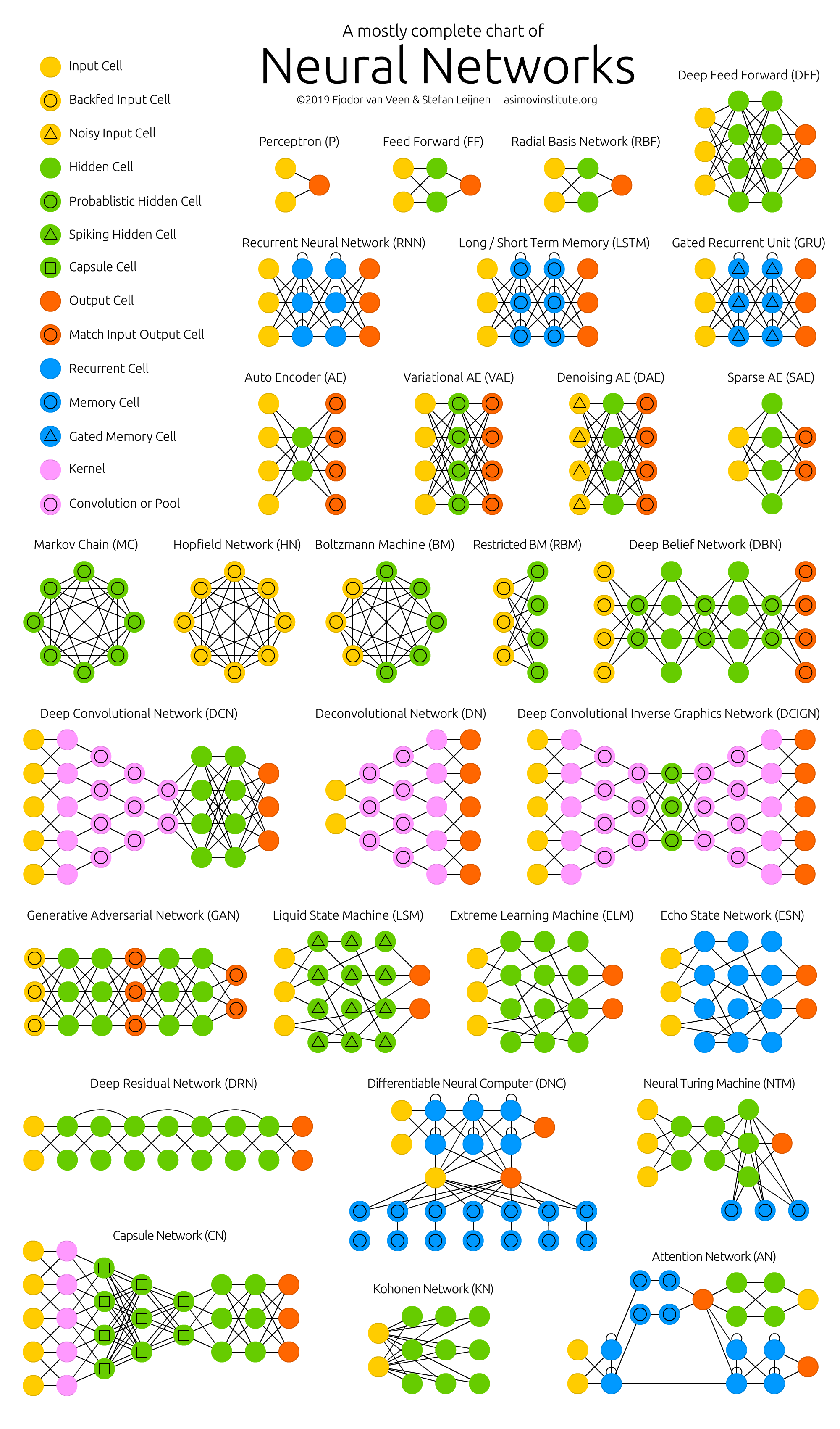
导读:这篇文章介绍了各种人工神经网络的结构,用图形形式展示了主流网络的基本结构类型。
本文总结的主要要点包括:
>> 介绍和归类了各种常见的人工神经网络架构,包括前馈神经网络、径向基函数网络、递归神经网络、长短期记忆网络、门控递归单元、卷积神经网络等等。
>> 对每种网络类型给出了简要生动的描述,分解网络结构,强调特征。
>> 给每个网络配有代表性的结构示意图,便于理解和区分不同类型的网络。
>> 提供很多原始论文链接,方便读者了解网络的最新研究进展。
>> 文章采用简洁明了的语言和结构,很好地总结概括了深度学习领域各种主流网络,帮助读者对网络有一个系统的认识。
这篇文章解决的痛点是,深度学习领域新网络层出不穷,很难对各种网络有一个清晰的认识。通过分类和图形形式总结不同网络的特点,这篇文章很好地解决了这个问题,帮助读者理解主流网络之间的联系和差异。此外,给出的原始论文链接,也推动读者深入学习网络的本质原理。
所以,这篇文章通过分类介绍、图解结构以及提供参考文献,极大地简化了读者理解各种人工神经网络的难点,起到很好的教学和总结作用。
目录
相关文章
《The Neural Network Zoo神经网络模型集合与分类》翻译与解读
Introduce
Neural Network Zoo
1、1958,P→FFNN
1988,RBF(Radial Basis Function)
2、1990,RNN
1997,LSTM
2014,GRU
1997,BiRNN→BiLSTM→BiGRU
3、1988,AE(AutoEncoders)
2013,VAE(Variational AutoEncoders)
2008,DAE(Denoising AutoEncoders)
2007,SAE(Sparse AutoEncoders)
4、2013,MC(Markov Chains)、DTMC
1982,HN(Hopfield Network )
1986,BM(Boltzmann Machines)
1986,RBM(Restricted Boltzmann Machines )
2007,DBN(Deep Belief Networks)
5、1998,CNN
2010,DN(Deconvolutional Networks)
2015,DCIGN(Deep Convolutional Inverse Graphics Networks )
6、2014,GAN(Generative Adversarial Networks )
2002,LSM(Liquid State Machines)
2006,ELM(Extreme Learning Machines)
2004,ESN(Echo State Networks )
7、2015,DRN(Deep Residual Networks )
8、2014,NTM(Neural Turing Machines )
9、2016,DNC(Differentiable Neural Computers )
10、2017,CapsNet
11、1982,KN(Kohonen Networks)
12、2015,AN(Attention Networks)
相关文章
DL:深度学习算法(神经网络模型集合)概览之《THE NEURAL NETWORK ZOO》的中文解释和感悟(一)
DL:深度学习算法(神经网络模型集合)概览之《THE NEURAL NETWORK ZOO》的中文解释和感悟(二)
DL:深度学习算法(神经网络模型集合)概览之《THE NEURAL NETWORK ZOO》的中文解释和感悟(三)
DL:深度学习算法(神经网络模型集合)概览之《THE NEURAL NETWORK ZOO》的中文解释和感悟(四)
DL:深度学习算法(神经网络模型集合)概览之《THE NEURAL NETWORK ZOO》的中文解释和感悟(五)
DL:深度学习算法(神经网络模型集合)概览之《THE NEURAL NETWORK ZOO》的中文解释和感悟(六)
《The Neural Network Zoo神经网络模型集合与分类》翻译与解读
Introduce
| With new neural network architectures popping up every now and then, it’s hard to keep track of them all. Knowing all the abbreviations being thrown around (DCIGN, BiLSTM, DCGAN, anyone?) can be a bit overwhelming at first. So I decided to compose a cheat sheet containing many of those architectures. Most of these are neural networks, some are completely different beasts. Though all of these architectures are presented as novel and unique, when I drew the node structures… their underlying relations started to make more sense. | 随着新的神经网络架构的不断涌现,很难对它们进行跟踪。了解所有这些缩写(DCIGN、BiLSTM、DCGAN等)可能一开始会有点令人不知所措。 因此,我决定编写一个包含许多这些架构的备忘单。其中大多数是神经网络,有些是完全不同的体系。尽管所有这些架构都被呈现为新颖和独特,但当我绘制节点结构时,它们的基本关系开始变得更加明晰。 |
| One problem with drawing them as node maps: it doesn’t really show how they’re used. For example, variational autoencoders (VAE) may look just like autoencoders (AE), but the training process is actually quite different. The use-cases for trained networks differ even more, because VAEs are generators, where you insert noise to get a new sample. AEs, simply map whatever they get as input to the closest training sample they “remember”. I should add that this overview is in no way clarifying how each of the different node types work internally (but that’s a topic for another day). It should be noted that while most of the abbreviations used are generally accepted, not all of them are. RNNs sometimes refer to recursive neural networks, but most of the time they refer to recurrent neural networks. That’s not the end of it though, in many places you’ll find RNN used as placeholder for any recurrent architecture, including LSTMs, GRUs and even the bidirectional variants. AEs suffer from a similar problem from time to time, where VAEs and DAEs and the like are called simply AEs. Many abbreviations also vary in the amount of “N”s to add at the end, because you could call it a convolutional neural network but also simply a convolutional network (resulting in CNN or CN). | 将它们绘制为节点图的一个问题是它并不能真正展示它们是如何被使用的。例如,变分自编码器(VAE)可能看起来就像自编码器(AE),但训练过程实际上是非常不同的。经过训练的网络的用例甚至更加不同,因为VAE是生成器,您可以插入噪声以获得新样本。相比之下,AE仅将其输入映射到最接近的训练样本,它“记住”的样本。我应该补充一点,这个概述并没有说明每种不同的节点类型是如何在内部工作的(但这是另一个话题)。 应该指出的是,虽然大多数使用的缩写通常被接受,但并非全部。RNN有时指的是递归神经网络,但大多数时候指的是循环神经网络。然而,并非所有的情况都是这样,许多地方会使用RNN来替代任何循环体系结构,包括LSTM、GRU甚至双向变体。AE有时也存在类似的问题,其中VAE和DAE等被简单地称为AE。许多缩写的“N”的数量也有所不同,因为你可以称其为卷积神经网络,也可以简单地称其为卷积网络(导致CNN或CN)。 |
| Composing a complete list is practically impossible, as new architectures are invented all the time. Even if published it can still be quite challenging to find them even if you’re looking for them, or sometimes you just overlook some. So while this list may provide you with some insights into the world of AI, please, by no means take this list for being comprehensive; especially if you read this post long after it was written. For each of the architectures depicted in the picture, I wrote a very, very brief description. You may find some of these to be useful if you’re quite familiar with some architectures, but you aren’t familiar with a particular one. | 组成完整的列表几乎是不可能的,因为新的架构一直在不断被发明。即使已经发布,如果你在寻找它们,找到它们仍然可能是相当具有挑战性的,有时你可能只是忽略了一些。因此,尽管这个列表可能为您提供了一些有关AI世界的见解,请切勿认为这个列表是全面的,特别是如果您在很久以后阅读此帖子。 对于图中描述的每一个架构,我都写了一个非常非常简短的描述。如果您非常熟悉某些体系结构,但不熟悉某个特定的体系结构,那么您可能会发现其中一些很有用。 |
| Follow us on twitter for future updates and posts. We welcome comments and feedback, and thank you for reading! [Update 22 April 2019] Included Capsule Networks, Differentiable Neural Computers and Attention Networks to the Neural Network Zoo; Support Vector Machines are removed; updated links to original articles. The previous version of this post can be found here . Van Veen, F. & Leijnen, S. (2019). The Neural Network Zoo. Retrieved from https://www.asimovinstitute.org/neural-network-zoo | 关注我们的Twitter获取未来的更新和帖子。我们欢迎评论和反馈,感谢您的阅读! 【2019年4月22日更新】将Capsule Networks、可微分神经计算机和Attention Networks添加到神经网络动物园;删除支持向量机;更新到原始文章的链接。之前版本的帖子可以在这里找到。 Van Veen, F. & Leijnen, S.(2019)。神经网络动物园。检索自https://www.asimovinstitute.org/neural-network-zoo |
Neural Network Zoo
1、1958,P→FFNN

| Feed forward neural networks (FF or FFNN) and perceptrons (P) are very straight forward, they feed information from the front to the back (input and output, respectively). Neural networks are often described as having layers, where each layer consists of either input, hidden or output cells in parallel. A layer alone never has connections and in general two adjacent layers are fully connected (every neuron form one layer to every neuron to another layer). The simplest somewhat practical network has two input cells and one output cell, which can be used to model logic gates. One usually trains FFNNs through back-propagation, giving the network paired datasets of “what goes in” and “what we want to have coming out”. This is called supervised learning, as opposed to unsupervised learning where we only give it input and let the network fill in the blanks. The error being back-propagated is often some variation of the difference between the input and the output (like MSE or just the linear difference). Given that the network has enough hidden neurons, it can theoretically always model the relationship between the input and output. Practically their use is a lot more limited but they are popularly combined with other networks to form new networks. Rosenblatt, Frank. “The perceptron: a probabilistic model for information storage and organization in the brain.” Psychological review 65.6 (1958): 386. | 前馈神经网络(FF或FFNN)和感知器(P)是非常直接的,它们分别从前向后传递信息(输入和输出)。神经网络通常被描述为具有层,其中每一层都由输入、隐藏或输出单元并行组成。单独的一层从不具有连接,通常两个相邻的层是完全连接的(每个神经元从一层到另一层的每个神经元)。最简单但实用的网络具有两个输入单元和一个输出单元,可用于建模逻辑门。通常通过反向传播来训练FFNN,给网络配对的数据集“输入什么”和“我们想要输出什么”。这被称为监督学习,与非监督学习相反,在非监督学习中,我们只给它输入,让网络填补空白。反向传播的误差通常是输入与输出之间的差异的某种变体(如MSE或线性差异)。假设网络有足够的隐藏神经元,它在理论上始终可以模拟输入和输出之间的关系。实际上,它们的使用受到很大限制,但它们通常与其他网络结合以形成新网络。 Rosenblatt,弗兰克。感知器:大脑中信息存储和组织的概率模型心理评论65.6(1958):386。 |
1988,RBF(Radial Basis Function)

| Radial basis function (RBF) networks are FFNNs with radial basis functions as activation functions. There’s nothing more to it. Doesn’t mean they don’t have their uses, but most FFNNs with other activation functions don’t get their own name. This mostly has to do with inventing them at the right time. Broomhead, David S., and David Lowe. Radial basis functions, multi-variable functional interpolation and adaptive networks. No. RSRE-MEMO-4148. ROYAL SIGNALS AND RADAR ESTABLISHMENT MALVERN (UNITED KINGDOM), 1988. Original Paper PDF | 径向基函数(RBF)网络是以径向基函数作为激活函数的FFNN。除此之外没有更多内容。这并不意味着它们没有用处,但大多数具有其他激活函数的FFNN没有自己的名字。这主要与在正确的时间发明它们有关。 布鲁姆黑德,大卫·S·和大卫·洛。径向基函数,多变量函数插值和自适应网络。不。rsre -备忘录- 4148。皇家信号和雷达建立马尔文(联合王国),1988。 原始文件PDF |
2、1990,RNN

| Recurrent neural networks (RNN) are FFNNs with a time twist: they are not stateless; they have connections between passes, connections through time. Neurons are fed information not just from the previous layer but also from themselves from the previous pass. This means that the order in which you feed the input and train the network matters: feeding it “milk” and then “cookies” may yield different results compared to feeding it “cookies” and then “milk”. One big problem with RNNs is the vanishing (or exploding) gradient problem where, depending on the activation functions used, information rapidly gets lost over time, just like very deep FFNNs lose information in depth. Intuitively this wouldn’t be much of a problem because these are just weights and not neuron states, but the weights through time is actually where the information from the past is stored; if the weight reaches a value of 0 or 1 000 000, the previous state won’t be very informative. RNNs can in principle be used in many fields as most forms of data that don’t actually have a timeline (i.e. unlike sound or video) can be represented as a sequence. A picture or a string of text can be fed one pixel or character at a time, so the time dependent weights are used for what came before in the sequence, not actually from what happened x seconds before. In general, recurrent networks are a good choice for advancing or completing information, such as autocompletion. Elman, Jeffrey L. “Finding structure in time.” Cognitive science 14.2 (1990): 179-211. Original Paper PDF | 循环神经网络(RNN)是带有时间扭曲的FFNN:它们不是无状态的;它们在传递之间有连接,穿越时间的联系。神经元不仅从上一层获取信息,还从它们自己的上一个传递中获取信息。这意味着输入和训练网络的顺序很重要:与输入“饼干”然后“牛奶”相比,输入“饼干”然后“牛奶”可能会产生不同的结果。RNN的一个大问题是梯度消失(或爆炸)问题,这取决于所使用的激活函数,信息随时间迅速丧失,就像非常深的FFNN在深度上丧失信息一样。从直觉上看,这本不是什么大问题,因为这些只是权重,而不是神经元状态,但是时间上的权重实际上是存储过去信息的地方;如果权重达到0或1,000,000的值,先前的状态将不会提供很多信息。原则上,RNN可以在许多领域使用,因为大多数形式的数据实际上没有时间轴(例如,不像声音或视频),可以用序列表示。一张图片或一串文本可以一次输入一个像素或字符,因此时间依赖的权重用于序列中之前发生的内容,而不是实际发生在x秒前的内容。总的来说,循环网络是推进或完成信息的很好选择,比如自动完成。 Elman, Jeffrey L., <及时发现结构>认知科学14.2(1990):179-211。 原始文件PDF |
1997,LSTM
| Long / short term memory (LSTM) networks try to combat the vanishing / exploding gradient problem by introducing gates and an explicitly defined memory cell. These are inspired mostly by circuitry, not so much biology. Each neuron has a memory cell and three gates: input, output and forget. The function of these gates is to safeguard the information by stopping or allowing the flow of it. The input gate determines how much of the information from the previous layer gets stored in the cell. The output layer takes the job on the other end and determines how much of the next layer gets to know about the state of this cell. The forget gate seems like an odd inclusion at first but sometimes it’s good to forget: if it’s learning a book and a new chapter begins, it may be necessary for the network to forget some characters from the previous chapter. LSTMs have been shown to be able to learn complex sequences, such as writing like Shakespeare or composing primitive music. Note that each of these gates has a weight to a cell in the previous neuron, so they typically require more resources to run. Hochreiter, Sepp, and Jürgen Schmidhuber. “Long short-term memory.” Neural computation 9.8 (1997): 1735-1780. Original Paper PDF | 长短时记忆(LSTM)网络试图通过引入门和显式定义的记忆单元来解决梯度消失/爆炸问题。这些灵感主要来自电路,而不是生物学。每个神经元都有一个记忆单元和三个门:输入门、输出门和遗忘门。这些门的功能是通过阻止或允许信息的流动来保护信息。输入门决定有多少来自前一层的信息被存储在单元中。输出层负责在另一端确定有多少下一层能够了解该单元状态的信息。遗忘门一开始看起来很奇怪,但有时遗忘是有好处的:如果它正在学习一本书,新的一章开始了,网络可能有必要忘记前一章中的一些字符。已经证明LSTM能够学习复杂的序列,例如像莎士比亚写作或创作原始音乐。请注意,这些门中的每一个都与前一个神经元中的单元有一个权重,因此它们通常需要更多的资源来运行。 Hochreiter, Sepp和j<s:1> rgen Schmidhuber。“长短期记忆。”神经计算9.8(1997):1735-1780。 原始文件PDF |
2014,GRU
| Gated recurrent units (GRU) are a slight variation on LSTMs. They have one less gate and are wired slightly differently: instead of an input, output and a forget gate, they have an update gate. This update gate determines both how much information to keep from the last state and how much information to let in from the previous layer. The reset gate functions much like the forget gate of an LSTM but it’s located slightly differently. They always send out their full state, they don’t have an output gate. In most cases, they function very similarly to LSTMs, with the biggest difference being that GRUs are slightly faster and easier to run (but also slightly less expressive). In practice these tend to cancel each other out, as you need a bigger network to regain some expressiveness which then in turn cancels out the performance benefits. In some cases where the extra expressiveness is not needed, GRUs can outperform LSTMs. Chung, Junyoung, et al. “Empirical evaluation of gated recurrent neural networks on sequence modeling.” arXiv preprint arXiv:1412.3555 (2014). Original Paper PDF | 门控循环单元(GRU)是LSTM的轻微变体。它们少了一个门,并且连接方式也略有不同:它们没有输入、输出和遗忘门,而是有一个更新门。此更新门确定从上一个状态保留多少信息以及从前一层中放入多少信息。重置门的功能与LSTM的遗忘门类似,但位置略有不同。它们总是发送出它们的完整状态,没有输出门。在大多数情况下,它们的功能与LSTM非常相似,最大的区别是GRU稍微更快且更容易运行(但也稍微不太表达)。在实践中,这些倾向于互相抵消,因为为了恢复一些表达性能,您需要更大的网络,然后这反过来抵消了性能优势。在不需要额外表达性的某些情况下,GRU可以胜过LSTM。 Chung, Junyoung, et . <门控递归神经网络在序列建模上的经验评价>。[j] .中国农业大学学报(自然科学版):1412.3555(2014)。 原始文件PDF |
1997,BiRNN→BiLSTM→BiGRU
| Bidirectional recurrent neural networks, bidirectional long / short term memory networks and bidirectional gated recurrent units (BiRNN, BiLSTM and BiGRU respectively) are not shown on the chart because they look exactly the same as their unidirectional counterparts. The difference is that these networks are not just connected to the past, but also to the future. As an example, unidirectional LSTMs might be trained to predict the word “fish” by being fed the letters one by one, where the recurrent connections through time remember the last value. A BiLSTM would also be fed the next letter in the sequence on the backward pass, giving it access to future information. This trains the network to fill in gaps instead of advancing information, so instead of expanding an image on the edge, it could fill a hole in the middle of an image. Schuster, Mike, and Kuldip K. Paliwal. “Bidirectional recurrent neural networks.” IEEE Transactions on Signal Processing 45.11 (1997): 2673-2681. Original Paper PDF | 双向循环神经网络、双向长短时记忆网络和双向门控循环单元(BiRNN、BiLSTM和BiGRU)没有显示在图表上,因为它们看起来与它们的单向对应物完全相同。区别在于这些网络不仅连接到过去,还连接到未来。例如,单向LSTM可以通过一个接一个地输入字母来训练预测单词“fish”,其中随着时间的推移循环连接会记住最后一个值。BiLSTM在反向传播时还将在后向传递中提供序列的下一个字母,从而获得对未来信息的访问。这训练网络填补空白而不是推进信息,因此与在边缘上扩展图像不同,它可以填补图像中间的空洞。 舒斯特,迈克,Kuldip K. Paliwal。“双向循环神经网络。”信号处理学报(英文版)(1997):2673-2681。 原始文件PDF |
3、1988,AE(AutoEncoders)
| Autoencoders (AE) are somewhat similar to FFNNs as AEs are more like a different use of FFNNs than a fundamentally different architecture. The basic idea behind autoencoders is to encode information (as in compress, not encrypt) automatically, hence the name. The entire network always resembles an hourglass like shape, with smaller hidden layers than the input and output layers. AEs are also always symmetrical around the middle layer(s) (one or two depending on an even or odd amount of layers). The smallest layer(s) is|are almost always in the middle, the place where the information is most compressed (the chokepoint of the network). Everything up to the middle is called the encoding part, everything after the middle the decoding and the middle (surprise) the code. One can train them using backpropagation by feeding input and setting the error to be the difference between the input and what came out. AEs can be built symmetrically when it comes to weights as well, so the encoding weights are the same as the decoding weights. Bourlard, Hervé, and Yves Kamp. “Auto-association by multilayer perceptrons and singular value decomposition.” Biological cybernetics 59.4-5 (1988): 291-294. Original Paper PDF | 自编码器(AE)与FFNN相似,因为AE更像是FFNN的不同用途,而不是基本不同的体系结构。自编码器背后的基本思想是自动编码信息(即压缩,而不是加密),因此得名。整个网络始终呈现出类似沙漏的形状,中间隐藏层比输入和输出层小。AE也总是围绕中间层(一个或两个,具体取决于层数的奇偶性)对称。最小的层通常在中间,这是信息最压缩的地方(网络的瓶颈)。从头到中间的一切被称为编码部分,中间之后的一切是解码部分,中间(惊喜)是编码。可以通过反向传播进行训练,通过提供输入并将误差设置为输入与输出之间的差异来进行训练。在权重方面,AE也可以在对称方面构建,因此编码权重与解码权重相同。 波拉德,赫弗尔,和伊夫·坎普。“多层感知器与奇异值分解的自动关联”。生物控制论(1988):291-294。 原始文件PDF |
2013,VAE(Variational AutoEncoders)
| Variational autoencoders (VAE) have the same architecture as AEs but are “taught” something else: an approximated probability distribution of the input samples. It’s a bit back to the roots as they are bit more closely related to BMs and RBMs. They do however rely on Bayesian mathematics regarding probabilistic inference and independence, as well as a re-parametrisation trick to achieve this different representation. The inference and independence parts make sense intuitively, but they rely on somewhat complex mathematics. The basics come down to this: take influence into account. If one thing happens in one place and something else happens somewhere else, they are not necessarily related. If they are not related, then the error propagation should consider that. This is a useful approach because neural networks are large graphs (in a way), so it helps if you can rule out influence from some nodes to other nodes as you dive into deeper layers. Kingma, Diederik P., and Max Welling. “Auto-encoding variational bayes.” arXiv preprint arXiv:1312.6114 (2013). Original Paper PDF | 变分自编码器(VAE)与AE具有相同的架构,但“教”它们的是输入样本的近似概率分布。这有点回到了根源,因为它们与BMs和RBMs更紧密相关。然而,它们确实依赖于关于概率推断和独立性的贝叶斯数学,以及一种重新参数化技巧来实现这种不同的表示。推理和独立性部分在直观上是有道理的,但它们依赖于相当复杂的数学。基本原则是考虑影响。如果一件事在一个地方发生,而另一件事在另一个地方发生,它们未必相关。如果它们不相关,那么误差传播应该考虑到这一点。这是一种有用的方法,因为神经网络是大型图(在某种程度上),所以如果可以排除一些节点对其他节点的影响,这有助于深入挖掘更深层次的信息。 金玛,迪德里克·P,还有麦克斯·韦林。“自动编码变分贝叶斯。[j] .中国农业大学学报(自然科学版):1312.6114(2013)。 原始文件PDF |
2008,DAE(Denoising AutoEncoders)
| Denoising autoencoders (DAE) are AEs where we don’t feed just the input data, but we feed the input data with noise (like making an image more grainy). We compute the error the same way though, so the output of the network is compared to the original input without noise. This encourages the network not to learn details but broader features, as learning smaller features often turns out to be “wrong” due to it constantly changing with noise. Vincent, Pascal, et al. “Extracting and composing robust features with denoising autoencoders.” Proceedings of the 25th international conference on Machine learning. ACM, 2008. Original Paper PDF | 去噪自编码器(DAE)是AE的一种形式,我们不只是输入数据,而是给输入数据加噪声(比如让图像更有颗粒感)。然而,我们以相同的方式计算误差,因此网络的输出与没有噪声的原始输入进行比较。这鼓励网络不学习细节而学习更广泛的特征,因为由于噪声的不断变化,学习较小的特征通常会被认为是“错误”的。 Vincent, Pascal等。“用去噪自动编码器提取和组合鲁棒特征。”第25届机器学习国际会议论文集。ACM, 2008年。 原始文件PDF |
2007,SAE(Sparse AutoEncoders)
| Sparse autoencoders (SAE) are in a way the opposite of AEs. Instead of teaching a network to represent a bunch of information in less “space” or nodes, we try to encode information in more space. So instead of the network converging in the middle and then expanding back to the input size, we blow up the middle. These types of networks can be used to extract many small features from a dataset. If one were to train a SAE the same way as an AE, you would in almost all cases end up with a pretty useless identity network (as in what comes in is what comes out, without any transformation or decomposition). To prevent this, instead of feeding back the input, we feed back the input plus a sparsity driver. This sparsity driver can take the form of a threshold filter, where only a certain error is passed back and trained, the other error will be “irrelevant” for that pass and set to zero. In a way this resembles spiking neural networks, where not all neurons fire all the time (and points are scored for biological plausibility). Marc’Aurelio Ranzato, Christopher Poultney, Sumit Chopra, and Yann LeCun. “Efficient learning of sparse representations with an energy-based model.” Proceedings of NIPS. 2007. Original Paper PDF | 稀疏自编码器(SAE)在某种程度上与ae相反。我们不是教网络在更少的“空间”或节点中表示一堆信息,而是尝试在更多的空间中对信息进行编码。所以我们不是在中间收敛然后扩展回输入大小,而是把中间放大。这些类型的网络可用于从数据集中提取许多小特征。如果用同样的方法训练SAE和AE,在几乎所有情况下,你都会得到一个非常无用的恒等式网络(就像进来的就是出来的一样,没有任何转换或分解)。为了防止这种情况,我们不是反馈输入,而是反馈输入加上一个稀疏驱动程序。这个稀疏性驱动程序可以采用阈值过滤器的形式,其中只有一个特定的错误被传递并训练,其他错误将与该传递“无关”并设置为零。在某种程度上,这类似于脉冲神经网络,并不是所有的神经元都在每时每刻被激活(分数是根据生物合理性来打分的)。 Marc 'Aurelio Ranzato, Christopher Poultney, Sumit Chopra和Yann LeCun。“基于能量模型的稀疏表示的有效学习。”NIPS会议录。2007. 原始文件PDF |
4、2013,MC(Markov Chains)、DTMC
| Markov chains (MC or discrete time Markov Chain, DTMC) are kind of the predecessors to BMs and HNs. They can be understood as follows: from this node where I am now, what are the odds of me going to any of my neighbouring nodes? They are memoryless (i.e. Markov Property) which means that every state you end up in depends completely on the previous state. While not really a neural network, they do resemble neural networks and form the theoretical basis for BMs and HNs. MC aren’t always considered neural networks, as goes for BMs, RBMs and HNs. Markov chains aren’t always fully connected either. Hayes, Brian. “First links in the Markov chain.” American Scientist 101.2 (2013): 252. Original Paper PDF | 马尔可夫链(MC或离散时间马尔可夫链,DTMC)是bm和HNs的前身。它们可以理解为:从我现在所在的这个节点,我到达相邻节点的概率是多少?它们是无记忆的(即马尔可夫属性),这意味着你最终的每个状态都完全依赖于前一个状态。虽然不是真正的神经网络,但它们确实类似于神经网络,并构成了bm和hn的理论基础。与bm、rbm和hn一样,MC并不总是被认为是神经网络。马尔可夫链也不总是完全连接的。 海耶斯,布莱恩。"马尔可夫链的第一环"美国科学家(2013):252。 原始文件PDF |
1982,HN(Hopfield Network )
| A Hopfield network (HN) is a network where every neuron is connected to every other neuron; it is a completely entangled plate of spaghetti as even all the nodes function as everything. Each node is input before training, then hidden during training and output afterwards. The networks are trained by setting the value of the neurons to the desired pattern after which the weights can be computed. The weights do not change after this. Once trained for one or more patterns, the network will always converge to one of the learned patterns because the network is only stable in those states. Note that it does not always conform to the desired state (it’s not a magic black box sadly). It stabilises in part due to the total “energy” or “temperature” of the network being reduced incrementally during training. Each neuron has an activation threshold which scales to this temperature, which if surpassed by summing the input causes the neuron to take the form of one of two states (usually -1 or 1, sometimes 0 or 1). Updating the network can be done synchronously or more commonly one by one. If updated one by one, a fair random sequence is created to organise which cells update in what order (fair random being all options (n) occurring exactly once every n items). This is so you can tell when the network is stable (done converging), once every cell has been updated and none of them changed, the network is stable (annealed). These networks are often called associative memory because the converge to the most similar state as the input; if humans see half a table we can image the other half, this network will converge to a table if presented with half noise and half a table. Hopfield, John J. “Neural networks and physical systems with emergent collective computational abilities.” Proceedings of the national academy of sciences 79.8 (1982): 2554-2558. Original Paper PDF | Hopfield网络(HN)是一种每个神经元相互连接的网络;它是一盘完全纠缠在一起的意大利面,因为所有的节点都发挥着一切的作用。每个节点在训练前输入,训练时隐藏,训练后输出。通过将神经元的值设置为期望的模式来训练网络,然后可以计算权重。权重在这之后不会改变。一旦训练了一个或多个模式,网络将总是收敛到其中一个学习模式,因为网络只有在那些状态下才稳定。请注意,它并不总是符合期望的状态(遗憾的是,它不是一个神奇的黑盒)。它的稳定部分是由于网络的总“能量”或“温度”在训练过程中逐渐减少。每个神经元都有一个激活阈值,该阈值可根据温度进行缩放,如果输入之和超过该阈值,则会导致神经元采取两种状态之一的形式(通常是-1或1,有时是0或1)。更新网络可以同步完成,也可以一个接一个地完成。如果逐个更新,将创建一个公平随机序列来组织哪些单元格以什么顺序更新(公平随机是所有选项(n)每n个项目恰好发生一次)。这样你就可以判断网络何时是稳定的(完成收敛),一旦每个单元都被更新并且它们都没有改变,网络就稳定了(退火)。这些网络通常被称为联想记忆,因为它们收敛到与输入最相似的状态;如果人类看到半张桌子,我们可以想象另一半,如果呈现一半噪音和一半桌子,这个网络将收敛到一张桌子。 Hopfield, John J., <具有涌现集体计算能力的神经网络和物理系统>国家科学院学报79.8(1982):2554-2558。 原始文件PDF |
1986,BM(Boltzmann Machines)
| Boltzmann machines (BM) are a lot like HNs, but: some neurons are marked as input neurons and others remain “hidden”. The input neurons become output neurons at the end of a full network update. It starts with random weights and learns through back-propagation, or more recently through contrastive divergence (a Markov chain is used to determine the gradients between two informational gains). Compared to a HN, the neurons mostly have binary activation patterns. As hinted by being trained by MCs, BMs are stochastic networks. The training and running process of a BM is fairly similar to a HN: one sets the input neurons to certain clamped values after which the network is set free (it doesn’t get a sock). While free the cells can get any value and we repetitively go back and forth between the input and hidden neurons. The activation is controlled by a global temperature value, which if lowered lowers the energy of the cells. This lower energy causes their activation patterns to stabilise. The network reaches an equilibrium given the right temperature. Hinton, Geoffrey E., and Terrence J. Sejnowski. “Learning and releaming in Boltzmann machines.” Parallel distributed processing: Explorations in the microstructure of cognition 1 (1986): 282-317. Original Paper PDF | 玻尔兹曼机(BM)与HNs非常相似,但是:一些神经元被标记为输入神经元,而其他神经元仍然“隐藏”。在一个完整的网络更新结束时,输入神经元变成了输出神经元。它从随机权重开始,通过反向传播学习,或者最近通过对比散度学习(使用马尔可夫链来确定两个信息增益之间的梯度)。与HN相比,神经元大多具有二元激活模式。正如mc所训练的那样,bm是随机网络。BM的训练和运行过程与HN非常相似:一个人将输入神经元设置为特定的固定值,之后网络就被释放了(它不会得到袜子)。在自由的时候,细胞可以得到任何值,我们在输入神经元和隐藏神经元之间反复地来回移动。激活是由一个全局温度值控制的,如果温度值降低,细胞的能量就会降低。这种较低的能量使它们的激活模式稳定下来。在适当的温度下,网络达到平衡。 Geoffrey E. Hinton和Terrence J. Sejnowski。"玻尔兹曼机器的学习和释放"并行分布式处理:认知微观结构的探索1(1986):282-317。 原始文件PDF |
1986,RBM(Restricted Boltzmann Machines )
| Restricted Boltzmann machines (RBM) are remarkably similar to BMs (surprise) and therefore also similar to HNs. The biggest difference between BMs and RBMs is that RBMs are a better usable because they are more restricted. They don’t trigger-happily connect every neuron to every other neuron but only connect every different group of neurons to every other group, so no input neurons are directly connected to other input neurons and no hidden to hidden connections are made either. RBMs can be trained like FFNNs with a twist: instead of passing data forward and then back-propagating, you forward pass the data and then backward pass the data (back to the first layer). After that you train with forward-and-back-propagation. Smolensky, Paul. Information processing in dynamical systems: Foundations of harmony theory. No. CU-CS-321-86. COLORADO UNIV AT BOULDER DEPT OF COMPUTER SCIENCE, 1986. Original Paper PDF | 受限玻尔兹曼机(RBM)与bm非常相似,因此也与hn相似。bm和rbm之间最大的区别是rbm的可用性更好,因为它们更受限制。它们并不是将每个神经元连接到另一个神经元,而是将每个不同的神经元组连接到另一个神经元组,所以没有输入神经元直接连接到其他输入神经元,也没有隐藏的连接到隐藏的连接。rbm可以像ffnn一样进行训练:不是向前传递数据然后反向传播,而是向前传递数据然后向后传递数据(回到第一层)。在那之后,你进行前向和反向传播训练。 Smolensky,保罗。动态系统中的信息处理:和谐理论的基础。不。铜- cs - 321 - 86。科罗拉多大学博尔德分校计算机科学系,1986年。 原始文件PDF |
2007,DBN(Deep Belief Networks)
| Deep belief networks (DBN) is the name given to stacked architectures of mostly RBMs or VAEs. These networks have been shown to be effectively trainable stack by stack, where each AE or RBM only has to learn to encode the previous network. This technique is also known as greedy training, where greedy means making locally optimal solutions to get to a decent but possibly not optimal answer. DBNs can be trained through contrastive divergence or back-propagation and learn to represent the data as a probabilistic model, just like regular RBMs or VAEs. Once trained or converged to a (more) stable state through unsupervised learning, the model can be used to generate new data. If trained with contrastive divergence, it can even classify existing data because the neurons have been taught to look for different features. Bengio, Yoshua, et al. “Greedy layer-wise training of deep networks.” Advances in neural information processing systems 19 (2007): 153. Original Paper PDF | 深度信念网络(DBN)是一种主要由rbm或vee组成的堆叠架构。这些网络已被证明是可有效地逐层训练的,其中每个AE或RBM只需学习对前一个网络进行编码。这种技术也被称为贪心训练,贪心意味着通过局部最优解来得到一个体面但可能不是最优的答案。dbn可以通过对比发散或反向传播进行训练,并学习将数据表示为概率模型,就像常规rbm或vae一样。一旦通过无监督学习训练或收敛到一个(更)稳定的状态,该模型就可以用来生成新的数据。如果用对比散度进行训练,它甚至可以对现有数据进行分类,因为神经元已经学会了寻找不同的特征。 Bengio, Yoshua等,“深度网络的贪婪分层训练。”神经信息处理系统进展[j](2007): 153。 原始文件PDF |
5、1998,CNN
| Convolutional neural networks (CNN or deep convolutional neural networks, DCNN) are quite different from most other networks. They are primarily used for image processing but can also be used for other types of input such as as audio. A typical use case for CNNs is where you feed the network images and the network classifies the data, e.g. it outputs “cat” if you give it a cat picture and “dog” when you give it a dog picture. CNNs tend to start with an input “scanner” which is not intended to parse all the training data at once. For example, to input an image of 200 x 200 pixels, you wouldn’t want a layer with 40 000 nodes. Rather, you create a scanning input layer of say 20 x 20 which you feed the first 20 x 20 pixels of the image (usually starting in the upper left corner). Once you passed that input (and possibly use it for training) you feed it the next 20 x 20 pixels: you move the scanner one pixel to the right. Note that one wouldn’t move the input 20 pixels (or whatever scanner width) over, you’re not dissecting the image into blocks of 20 x 20, but rather you’re crawling over it. This input data is then fed through convolutional layers instead of normal layers, where not all nodes are connected to all nodes. Each node only concerns itself with close neighbouring cells (how close depends on the implementation, but usually not more than a few). These convolutional layers also tend to shrink as they become deeper, mostly by easily divisible factors of the input (so 20 would probably go to a layer of 10 followed by a layer of 5). Powers of two are very commonly used here, as they can be divided cleanly and completely by definition: 32, 16, 8, 4, 2, 1. Besides these convolutional layers, they also often feature pooling layers. Pooling is a way to filter out details: a commonly found pooling technique is max pooling, where we take say 2 x 2 pixels and pass on the pixel with the most amount of red. To apply CNNs for audio, you basically feed the input audio waves and inch over the length of the clip, segment by segment. Real world implementations of CNNs often glue an FFNN to the end to further process the data, which allows for highly non-linear abstractions. These networks are called DCNNs but the names and abbreviations between these two are often used interchangeably. LeCun, Yann, et al. “Gradient-based learning applied to document recognition.” Proceedings of the IEEE 86.11 (1998): 2278-2324. Original Paper PDF | 卷积神经网络(CNN或深度卷积神经网络,DCNN)与大多数其他网络有很大的区别。它们主要用于图像处理,但也可以用于其他类型的输入,比如音频。CNN的典型用例是将图像输入网络,然后网络对数据进行分类,例如,如果你给它一张猫的图片,它会输出“cat”,如果给它一张狗的图片,它会输出“dog”。CNN通常以一个输入“扫描器”开始,该扫描器并不打算一次解析所有训练数据。例如,要输入一张200 x 200像素的图像,你不希望有一层有40000个节点。相反,你创建一个扫描输入层,比如20 x 20,然后将图像的前20 x 20像素馈送给它(通常从左上角开始)。一旦通过了这个输入(可能用于训练),你就将下一个20 x 20像素馈送给它:移动扫描器一个像素到右边。注意,你不会将输入移动20个像素(或任何扫描器宽度),你不是将图像分解成20 x 20的块,而是在其上爬行。然后,将这个输入数据通过卷积层而不是正常层进行馈送,在普通层中,并非所有节点都与所有节点相连接。每个节点只关注附近的单元(接近程度取决于实现,但通常不超过几个)。这些卷积层在深度增加时也往往会缩小,主要是通过输入的容易可分割的因子(因此20可能会变成10,然后是5)。这里非常常用2的幂,因为它们可以清晰完整地被定义分割:32、16、8、4、2、1。除了这些卷积层,它们通常还包括池化层。池化是一种过滤细节的方法:常见的池化技术是最大池化,我们取例如2 x 2的像素,并传递具有最多红色的像素。要将CNN用于音频,基本上是将输入音频波形馈送进去,并沿着剪辑的长度逐段进行。实际应用中,CNN的实现通常在最后连接一个前馈神经网络(FFNN)来进一步处理数据,这允许进行高度非线性的抽象。这些网络被称为DCNNs,但这两者之间的名称和缩写通常是可互换使用的。 LeCun, Yann等。“基于梯度的学习应用于文档识别。”电子工程学报(英文版)(1998):2278-2324。 原始文件PDF |
2010,DN(Deconvolutional Networks)
| Deconvolutional networks (DN), also called inverse graphics networks (IGNs), are reversed convolutional neural networks. Imagine feeding a network the word “cat” and training it to produce cat-like pictures, by comparing what it generates to real pictures of cats. DNNs can be combined with FFNNs just like regular CNNs, but this is about the point where the line is drawn with coming up with new abbreviations. They may be referenced as deep deconvolutional neural networks, but you could argue that when you stick FFNNs to the back and the front of DNNs that you have yet another architecture which deserves a new name. Note that in most applications one wouldn’t actually feed text-like input to the network, more likely a binary classification input vector. Think <0, 1> being cat, <1, 0> being dog and <1, 1> being cat and dog. The pooling layers commonly found in CNNs are often replaced with similar inverse operations, mainly interpolation and extrapolation with biased assumptions (if a pooling layer uses max pooling, you can invent exclusively lower new data when reversing it). Zeiler, Matthew D., et al. “Deconvolutional networks.” Computer Vision and Pattern Recognition (CVPR), 2010 IEEE Conference on. IEEE, 2010. Original Paper PDF | 反卷积网络(DN),也称为逆图形网络(ign),是一种反向卷积神经网络。想象一下,给一个网络输入“猫”这个词,并通过将其生成的图像与真实的猫的图像进行比较,训练它生成类似猫的图像。dnn可以与ffnn结合,就像普通的cnn一样,但这是关于提出新缩写的界限。它们可能被称为深度反卷积神经网络,但你可能会说,当你把ffnn放在dnn的后面和前面时,你就有了另一个值得新名字的架构。请注意,在大多数应用程序中,实际上不会向网络提供类似文本的输入,而更可能是二进制分类输入向量。想象< 0,1 >是猫,< 1,0 >是狗,< 1,1 >是猫和狗。在cnn中常见的池化层经常被类似的逆操作所取代,主要是带有偏见假设的插值和外推(如果池化层使用最大池化,你可以在反转它时专门发明更低的新数据)。 Zeiler, Matthew D.等人,《反卷积网络》。计算机视觉与模式识别(CVPR), 2010年IEEE学术会议。IEEE 2010。 原始文件PDF |
2015,DCIGN(Deep Convolutional Inverse Graphics Networks )
| Deep convolutional inverse graphics networks (DCIGN) have a somewhat misleading name, as they are actually VAEs but with CNNs and DNNs for the respective encoders and decoders. These networks attempt to model “features” in the encoding as probabilities, so that it can learn to produce a picture with a cat and a dog together, having only ever seen one of the two in separate pictures. Similarly, you could feed it a picture of a cat with your neighbours’ annoying dog on it, and ask it to remove the dog, without ever having done such an operation. Demo’s have shown that these networks can also learn to model complex transformations on images, such as changing the source of light or the rotation of a 3D object. These networks tend to be trained with back-propagation. Kulkarni, Tejas D., et al. “Deep convolutional inverse graphics network.” Advances in Neural Information Processing Systems. 2015. Original Paper PDF | 深度卷积逆图形网络(DCIGN)有一个有点误导人的名字,因为它们实际上是VAEs,但分别使用cnn和dnn作为编码器和解码器。这些网络试图将编码中的“特征”建模为概率,这样它就可以学习生成猫和狗在一起的图片,而只在单独的图片中看到过两者中的一个。类似地,你可以给它喂一张猫的照片,上面有你邻居的讨厌狗,然后让它把狗移走,而不需要做这样的手术。演示表明,这些网络还可以学习对图像进行复杂变换的建模,例如改变光源或3D物体的旋转。这些网络倾向于用反向传播来训练。 Kulkarni, Tejas D.等,“深度卷积逆图形网络”。神经信息处理系统进展。2015。 原始文件PDF |
6、2014,GAN(Generative Adversarial Networks )
| Generative adversarial networks (GAN) are from a different breed of networks, they are twins: two networks working together. GANs consist of any two networks (although often a combination of FFs and CNNs), with one tasked to generate content and the other has to judge content. The discriminating network receives either training data or generated content from the generative network. How well the discriminating network was able to correctly predict the data source is then used as part of the error for the generating network. This creates a form of competition where the discriminator is getting better at distinguishing real data from generated data and the generator is learning to become less predictable to the discriminator. This works well in part because even quite complex noise-like patterns are eventually predictable but generated content similar in features to the input data is harder to learn to distinguish. GANs can be quite difficult to train, as you don’t just have to train two networks (either of which can pose it’s own problems) but their dynamics need to be balanced as well. If prediction or generation becomes to good compared to the other, a GAN won’t converge as there is intrinsic divergence. Goodfellow, Ian, et al. “Generative adversarial nets.” Advances in Neural Information Processing Systems (2014). Original Paper PDF | 生成对抗网络(GAN)来自不同种类的网络,它们是双胞胎:两个网络一起工作。gan由任意两个网络组成(尽管通常是ff和cnn的组合),其中一个负责生成内容,另一个负责判断内容。鉴别网络接收来自生成网络的训练数据或生成内容。判别网络正确预测数据源的能力,然后作为生成网络误差的一部分。这创造了一种竞争形式,即判别器在区分真实数据和生成数据方面做得越来越好,而生成器则在学习变得越来越难以预测。这在一定程度上很有效,因为即使是非常复杂的噪声模式最终也是可预测的,但生成的内容与输入数据的特征相似,很难学会区分。gan可能很难训练,因为你不仅需要训练两个网络(其中任何一个都可能带来自己的问题),而且它们的动态也需要平衡。如果预测或生成变得比另一个好,GAN将不会收敛,因为存在固有的散度。 Goodfellow, Ian等人,《生成对抗网络》。神经信息处理系统进展(2014)。 原始文件PDF |
2002,LSM(Liquid State Machines)
| Liquid state machines (LSM) are similar soups, looking a lot like ESNs. The real difference is that LSMs are a type of spiking neural networks: sigmoid activations are replaced with threshold functions and each neuron is also an accumulating memory cell. So when updating a neuron, the value is not set to the sum of the neighbours, but rather added to itself. Once the threshold is reached, it releases its’ energy to other neurons. This creates a spiking like pattern, where nothing happens for a while until a threshold is suddenly reached. Maass, Wolfgang, Thomas Natschläger, and Henry Markram. “Real-time computing without stable states: A new framework for neural computation based on perturbations.” Neural computation 14.11 (2002): 2531-2560. Original Paper PDF | 液态机(LSM)是类似的汤,看起来很像esn。真正的区别在于lsm是一种尖峰神经网络:s形激活被阈值函数取代,每个神经元也是一个累积记忆细胞。因此,当更新一个神经元时,值不是设置为邻居的和,而是添加到自身。一旦达到阈值,它就会将能量释放给其他神经元。这就形成了一个尖峰式的模式,在一段时间内什么都没有发生,直到突然达到一个阈值。 马斯,沃尔夫冈,托马斯Natschläger,还有亨利·马克拉姆。无稳定状态的实时计算:基于扰动的神经计算新框架。神经计算14(2002):2531-2560。 原始文件PDF |
2006,ELM(Extreme Learning Machines)
| Extreme learning machines (ELM) are basically FFNNs but with random connections. They look very similar to LSMs and ESNs, but they are not recurrent nor spiking. They also do not use backpropagation. Instead, they start with random weights and train the weights in a single step according to the least-squares fit (lowest error across all functions). This results in a much less expressive network but it’s also much faster than backpropagation. Huang, Guang-Bin, et al. “Extreme learning machine: Theory and applications.” Neurocomputing 70.1-3 (2006): 489-501. Original Paper PDF | 极限学习机(ELM)基本上是带有随机连接的ffnn。它们看起来与lsm和ESNs非常相似,但它们既不复发也不尖峰。它们也不使用反向传播。相反,它们从随机权重开始,并根据最小二乘拟合(所有函数的最小误差)在单个步骤中训练权重。这导致网络的表达能力大大降低,但也比反向传播快得多。 黄光斌,等。“极限学习机:理论与应用”。神经计算机学报(英文版)(2006):489- 491。 原始文件PDF |
2004,ESN(Echo State Networks )
| Echo state networks (ESN) are yet another different type of (recurrent) network. This one sets itself apart from others by having random connections between the neurons (i.e. not organised into neat sets of layers), and they are trained differently. Instead of feeding input and back-propagating the error, we feed the input, forward it and update the neurons for a while, and observe the output over time. The input and the output layers have a slightly unconventional role as the input layer is used to prime the network and the output layer acts as an observer of the activation patterns that unfold over time. During training, only the connections between the observer and the (soup of) hidden units are changed. Jaeger, Herbert, and Harald Haas. “Harnessing nonlinearity: Predicting chaotic systems and saving energy in wireless communication.” science 304.5667 (2004): 78-80. Original Paper PDF | 回声状态网络(ESN)是另一种不同类型的(循环)网络。这种神经元通过神经元之间的随机连接(即没有组织成整齐的层集)将自己与其他神经元区分开来,并且它们的训练方式不同。我们不是输入输入然后反向传播误差,而是输入输入,转发并更新神经元一段时间,然后观察一段时间后的输出。输入层和输出层的作用略显非常规,因为输入层用于启动网络,而输出层则充当随时间展开的激活模式的观察者。在训练过程中,只有观察者和隐藏单位之间的连接被改变。 耶格,赫伯特和哈拉尔德·哈斯。利用非线性:预测无线通信中的混沌系统和节能。science 304.5667(2004): 78-80。 原始文件PDF |
7、2015,DRN(Deep Residual Networks )
| Deep residual networks (DRN) are very deep FFNNs with extra connections passing input from one layer to a later layer (often 2 to 5 layers) as well as the next layer. Instead of trying to find a solution for mapping some input to some output across say 5 layers, the network is enforced to learn to map some input to some output + some input. Basically, it adds an identity to the solution, carrying the older input over and serving it freshly to a later layer. It has been shown that these networks are very effective at learning patterns up to 150 layers deep, much more than the regular 2 to 5 layers one could expect to train. However, it has been proven that these networks are in essence just RNNs without the explicit time based construction and they’re often compared to LSTMs without gates. He, Kaiming, et al. “Deep residual learning for image recognition.” arXiv preprint arXiv:1512.03385 (2015). Original Paper PDF | 深度残差网络(DRN)是非常深的ffnn,具有将输入从一层传递到下一层(通常为2到5层)以及下一层的额外连接。而不是试图找到一个解决方案,将一些输入映射到一些输出,跨越5层,网络被迫学习将一些输入映射到一些输出+一些输入。基本上,它为解决方案添加了一个身份,将旧的输入传递给后一层,并将其新鲜地提供给后一层。研究表明,这些网络在学习高达150层深度的模式方面非常有效,远远超过人们期望训练的常规2到5层。然而,事实证明,这些网络本质上只是rnn,没有明确的基于时间的结构,它们经常被比作没有门的lstm。 何凯明等,“图像识别的深度残差学习。”arXiv预印本arXiv:1512.03385(2015)。 原始文件PDF |
8、2014,NTM(Neural Turing Machines )
| Neural Turing machines (NTM) can be understood as an abstraction of LSTMs and an attempt to un-black-box neural networks (and give us some insight in what is going on in there). Instead of coding a memory cell directly into a neuron, the memory is separated. It’s an attempt to combine the efficiency and permanency of regular digital storage and the efficiency and expressive power of neural networks. The idea is to have a content-addressable memory bank and a neural network that can read and write from it. The “Turing” in Neural Turing Machines comes from them being Turing complete: the ability to read and write and change state based on what it reads means it can represent anything a Universal Turing Machine can represent. Graves, Alex, Greg Wayne, and Ivo Danihelka. “Neural turing machines.” arXiv preprint arXiv:1410.5401 (2014). Original Paper PDF | 神经图灵机(Neural Turing machines, NTM)可以理解为lstm的一个抽象,并且是对非黑盒神经网络的一种尝试(并让我们对其中发生的事情有一些了解)。不是将记忆细胞直接编码到神经元中,而是将记忆分离。它试图将常规数字存储的效率和持久性与神经网络的效率和表达能力结合起来。这个想法是有一个内容可寻址的记忆库和一个可以从中读写的神经网络。神经图灵机中的“图灵”来自于它们是图灵完备的:读写和根据读取的内容改变状态的能力意味着它可以表示通用图灵机可以表示的任何东西。 格雷夫斯,亚历克斯,格雷格·韦恩,还有伊沃·达尼赫尔卡。“神经图灵机。[j] .中国科学院学报(自然科学版):1410.5401(2014)。 原始文件PDF |
9、2016,DNC(Differentiable Neural Computers )
| Differentiable Neural Computers (DNC) are enhanced Neural Turing Machines with scalable memory, inspired by how memories are stored by the human hippocampus. The idea is to take the classical Von Neumann computer architecture and replace the CPU with an RNN, which learns when and what to read from the RAM. Besides having a large bank of numbers as memory (which may be resized without retraining the RNN). The DNC also has three attention mechanisms. These mechanisms allow the RNN to query the similarity of a bit of input to the memory’s entries, the temporal relationship between any two entries in memory, and whether a memory entry was recently updated – which makes it less likely to be overwritten when there’s no empty memory available. Graves, Alex, et al. “Hybrid computing using a neural network with dynamic external memory.” Nature 538 (2016): 471-476. Original Paper PDF | 可微分神经计算机(DNC)是具有可扩展记忆的增强型神经图灵机,其灵感来自于人类海马体存储记忆的方式。这个想法是采用经典的冯·诺伊曼计算机体系结构,用RNN取代CPU, RNN学习何时从RAM读取以及读取什么内容。除了拥有大量的数字作为内存(可以在不重新训练RNN的情况下调整大小)。民主党全国委员会还有三种关注机制。这些机制允许RNN查询一些输入与内存条目的相似性,内存中任意两个条目之间的时间关系,以及内存条目最近是否更新-这使得当没有空内存可用时,它不太可能被覆盖。 Graves, Alex等人,《使用带有动态外部存储器的神经网络的混合计算》。《自然》(2016):471-476。 原始文件PDF |
10、2017,CapsNet
| Capsule Networks (CapsNet) are biology inspired alternatives to pooling, where neurons are connected with multiple weights (a vector) instead of just one weight (a scalar). This allows neurons to transfer more information than simply which feature was detected, such as where a feature is in the picture or what colour and orientation it has. The learning process involves a local form of Hebbian learning that values correct predictions of output in the next layer. Sabour, Sara, Frosst, Nicholas, and Hinton, G. E. “Dynamic Routing Between Capsules.” In Advances in neural information processing systems (2017): 3856-3866. Original Paper PDF | 胶囊网络(CapsNet)是受生物学启发的池化替代方案,其中神经元与多个权重(矢量)连接,而不仅仅是一个权重(标量)。这使得神经元能够传递更多的信息,而不仅仅是检测到哪个特征,比如一个特征在图片中的位置,或者它的颜色和方向。学习过程涉及一种局部形式的Hebbian学习,它重视对下一层输出的正确预测。 Sabour, Sara, frost, Nicholas和Hinton, g.e.《胶囊之间的动态路由》。神经信息处理系统研究进展(2017):3856-3866。 原始文件PDF |
11、1982,KN(Kohonen Networks)
| Kohonen networks (KN, also self organising (feature) map, SOM, SOFM) utilise competitive learning to classify data without supervision. Input is presented to the network, after which the network assesses which of its neurons most closely match that input. These neurons are then adjusted to match the input even better, dragging along their neighbours in the process. How much the neighbours are moved depends on the distance of the neighbours to the best matching units. Kohonen, Teuvo. “Self-organized formation of topologically correct feature maps.” Biological cybernetics 43.1 (1982): 59-69. Original Paper PDF | Kohonen网络(KN,也称为自组织(特征)图、SOM、SOFM)利用竞争学习在没有监督的情况下对数据进行分类。输入被呈现给网络,然后网络评估哪个神经元与输入最匹配。然后,这些神经元被调整以更好地匹配输入,在这个过程中拖着它们的邻居。邻居的移动程度取决于邻居到最佳匹配单元的距离。 Kohonen Teuvo。“拓扑正确特征图的自组织形成。”生物控制论43.1(1982):59-69。 原始文件PDF |
12、2015,AN(Attention Networks)
| Attention networks (AN) can be considered a class of networks, which includes the Transformer architecture. They use an attention mechanism to combat information decay by separately storing previous network states and switching attention between the states. The hidden states of each iteration in the encoding layers are stored in memory cells. The decoding layers are connected to the encoding layers, but it also receives data from the memory cells filtered by an attention context. This filtering step adds context for the decoding layers stressing the importance of particular features. The attention network producing this context is trained using the error signal from the output of decoding layer. Moreover, the attention context can be visualized giving valuable insight into which input features correspond with what output features. Jaderberg, Max, et al. “Spatial Transformer Networks.” In Advances in neural information processing systems (2015): 2017-2025. Original Paper PDF | 注意网络(AN)可以被认为是一类网络,它包括Transformer体系结构。他们使用一种注意力机制来对抗信息衰减,方法是分别存储以前的网络状态并在状态之间切换注意力。编码层中每次迭代的隐藏状态存储在存储单元中。解码层与编码层相连,但它也从经过注意上下文过滤的记忆细胞接收数据。这个过滤步骤为解码层增加了上下文,强调了特定特征的重要性。利用解码层输出的错误信号训练产生该上下文的注意网络。此外,注意上下文可以可视化,从而有价值地洞察哪些输入特征与哪些输出特征相对应。 Jaderberg, Max等人,<空间变压器网络>。神经信息处理系统进展(2015):2017-2025。 原始文件PDF |
这篇关于DL之DNN:《The Neural Network Zoo神经网络模型集合与分类》翻译与解读的文章就介绍到这儿,希望我们推荐的文章对编程师们有所帮助!


