本文主要是介绍软著项目推荐 深度学习卷积神经网络的花卉识别,希望对大家解决编程问题提供一定的参考价值,需要的开发者们随着小编来一起学习吧!
文章目录
- 0 前言
- 1 项目背景
- 2 花卉识别的基本原理
- 3 算法实现
- 3.1 预处理
- 3.2 特征提取和选择
- 3.3 分类器设计和决策
- 3.4 卷积神经网络基本原理
- 4 算法实现
- 4.1 花卉图像数据
- 4.2 模块组成
- 5 项目执行结果
- 6 最后
0 前言
🔥 优质竞赛项目系列,今天要分享的是
基于深度学习卷积神经网络的花卉识别
该项目较为新颖,适合作为竞赛课题方向,学长非常推荐!
🧿 更多资料, 项目分享:
https://gitee.com/dancheng-senior/postgraduate
1 项目背景
在我国有着成千上万种花卉, 但如何能方便快捷的识别辨识出这些花卉的种类成为了植物学领域的重要研究课题。 我国的花卉研究历史悠久,
是世界上研究较早的国家之一。 花卉是我国重要的物产资源, 除美化了环境, 调养身心外, 它还具有药用价值, 并且在医学领域为保障人们的健康起着重要作用。
花卉识别是植物学领域的一个重要课题, 多年来已经形成一定体系化分类系统,但需要植物学家耗费大量的精力人工分析。 这种方法要求我们首先去了解花卉的生长环境,
近而去研究花卉的整体形态特征。 在观察植株形态特征时尤其是重点观察花卉的花蕊特征、 花卉的纹理颜色和形状及其相关信息等。 然后在和现有的样本进行比对,
最终确定花卉的所属类别。
2 花卉识别的基本原理
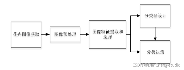
花卉种类识别功能实现的主要途径是利用计算机对样本进行分类。 通过对样本的精准分类达到得出图像识别结果的目的。 经典的花卉识别设计如下图 所示,
这几个过程相互关联而又有明显区别。
3 算法实现
3.1 预处理
预处理是对处于最低抽象级别的图像进行操作的通用名称, 输入和输出均为强度图像。 为了使实验结果更精准, 需要对图像数据进行预处理, 比如,
根据需要增强图像质量、 将图像裁剪成大小一致的形状、 避免不必要的失真等等。
3.2 特征提取和选择
要想获取花卉图像中的最具代表性的隐含信息, 就必须对花卉图像数据集进行相应的变换。
特征提取旨在通过从现有特征中创建新特征(然后丢弃原始特征) 来减少数据集中的特征数量。 然后, 这些新的简化功能集应该能够汇总原始功能集中包含的大多数信息。
这样, 可以从原始集合的组合中创建原始特征的摘要版本。 对所获取的信息实现从测量空间到特征空间的转换。
3.3 分类器设计和决策
构建完整系统的适当分类器组件的任务是使用特征提取器提供的特征向量将对象分配给类别。 由于完美的分类性能通常是不可能实现的,
因此一般的任务是确定每种可能类别的概率。 输入数据的特征向量表示所提供的抽象使得能够开发出在尽可能大程度上与领域无关的分类理论。
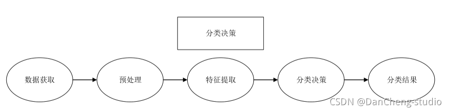

在设计阶段, 决策功能必须重复多次, 直到错误达到特定条件为止。 分类决策是在分类器设计阶段基于预处理、 特征提取与选择及判决函数建立的模型,
对接收到的样本数据进行归类, 然后输出分类结果。
3.4 卷积神经网络基本原理
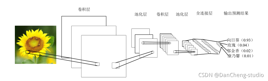
卷积神经网络是受到生物学启发的深度学习经典的多层前馈神经网络结构。 是一种在图像分类中广泛使用的机器学习算法。
CNN 的灵感来自我们人类实际看到并识别物体的方式。 这是基于一种方法,即我们眼睛中的神经元细胞只接收到整个对象的一小部分,而这些小块(称为接受场)
被组合在一起以形成整个对象。与其他的人工视觉算法不一样的是 CNN 可以处理特定任务的多个阶段的不变特征。
卷积神经网络使用的并不像经典的人工神经网络那样的全连接层, 而是通过采取局部连接和权值共享的方法, 来使训练的参数量减少, 降低模型的训练复杂度。
CNN 在图像分类和其他识别任务方面已经使传统技术的识别效果得到显著的改善。 由于在过去的几年中卷积网络的快速发展, 对象分类和目标检测能力取得喜人的成绩。
典型的 CNN 含有多个卷积层和池化层, 并具有全连接层以产生任务的最终结果。 在图像分类中, 最后一层的每个单元表示分类概率。
4 算法实现
4.1 花卉图像数据
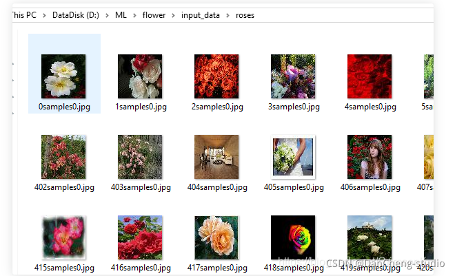
花卉图像的获取除了通过用拍摄设备手工收集或是通过网络下载已经整理好的现有数据集, 还可以通过网络爬虫技术收集整理自己的数据集。

以roses种类的训练数据为例,文件夹内部均为该种类花的图像文件
4.2 模块组成
示例代码主要由四个模块组成:
- input_data.py——图像特征提取模块,模块生成四种花的品类图片路径及对应标签的List
- model.py——模型模块,构建完整的CNN模型
- train.py——训练模块,训练模型,并保存训练模型结果
- test.py——测试模块,测试模型对图片识别的准确度
项目模块执行顺序
运行train.py开始训练。
训练完成后- 运行test.py,查看实际测试结果
input_data.py——图像特征提取模块,模块生成四种花的品类图片路径及对应标签的List
import os
import math
import numpy as np
import tensorflow as tf
import matplotlib.pyplot as plt# -----------------生成图片路径和标签的List------------------------------------
train_dir = 'D:/ML/flower/input_data'roses = []
label_roses = []
tulips = []
label_tulips = []
dandelion = []
label_dandelion = []
sunflowers = []
label_sunflowers = []
定义函数get_files,获取图片列表及标签列表
# step1:获取所有的图片路径名,存放到# 对应的列表中,同时贴上标签,存放到label列表中。def get_files(file_dir, ratio):for file in os.listdir(file_dir + '/roses'):roses.append(file_dir + '/roses' + '/' + file)label_roses.append(0)for file in os.listdir(file_dir + '/tulips'):tulips.append(file_dir + '/tulips' + '/' + file)label_tulips.append(1)for file in os.listdir(file_dir + '/dandelion'):dandelion.append(file_dir + '/dandelion' + '/' + file)label_dandelion.append(2)for file in os.listdir(file_dir + '/sunflowers'):sunflowers.append(file_dir + '/sunflowers' + '/' + file)label_sunflowers.append(3)# step2:对生成的图片路径和标签List做打乱处理image_list = np.hstack((roses, tulips, dandelion, sunflowers))label_list = np.hstack((label_roses, label_tulips, label_dandelion, label_sunflowers))# 利用shuffle打乱顺序temp = np.array([image_list, label_list])temp = temp.transpose()np.random.shuffle(temp)# 将所有的img和lab转换成listall_image_list = list(temp[:, 0])all_label_list = list(temp[:, 1])# 将所得List分为两部分,一部分用来训练tra,一部分用来测试val# ratio是测试集的比例n_sample = len(all_label_list)n_val = int(math.ceil(n_sample * ratio)) # 测试样本数n_train = n_sample - n_val # 训练样本数tra_images = all_image_list[0:n_train]tra_labels = all_label_list[0:n_train]tra_labels = [int(float(i)) for i in tra_labels]val_images = all_image_list[n_train:-1]val_labels = all_label_list[n_train:-1]val_labels = [int(float(i)) for i in val_labels]return tra_images, tra_labels, val_images, val_labels定义函数get_batch,生成训练批次数据
# --------------------生成Batch----------------------------------------------# step1:将上面生成的List传入get_batch() ,转换类型,产生一个输入队列queue,因为img和lab
# 是分开的,所以使用tf.train.slice_input_producer(),然后用tf.read_file()从队列中读取图像
#   image_W, image_H, :设置好固定的图像高度和宽度
#   设置batch_size:每个batch要放多少张图片
#   capacity:一个队列最大多少
定义函数get_batch,生成训练批次数据
def get_batch(image, label, image_W, image_H, batch_size, capacity):# 转换类型image = tf.cast(image, tf.string)label = tf.cast(label, tf.int32)# make an input queueinput_queue = tf.train.slice_input_producer([image, label])label = input_queue[1]image_contents = tf.read_file(input_queue[0])  # read img from a queue# step2:将图像解码,不同类型的图像不能混在一起,要么只用jpeg,要么只用png等。image = tf.image.decode_jpeg(image_contents, channels=3)# step3:数据预处理,对图像进行旋转、缩放、裁剪、归一化等操作,让计算出的模型更健壮。image = tf.image.resize_image_with_crop_or_pad(image, image_W, image_H)image = tf.image.per_image_standardization(image)# step4:生成batch# image_batch: 4D tensor [batch_size, width, height, 3],dtype=tf.float32# label_batch: 1D tensor [batch_size], dtype=tf.int32image_batch, label_batch = tf.train.batch([image, label],batch_size=batch_size,num_threads=32,capacity=capacity)# 重新排列label,行数为[batch_size]label_batch = tf.reshape(label_batch, [batch_size])image_batch = tf.cast(image_batch, tf.float32)return image_batch, label_batch
model.py——CN模型构建
import tensorflow as tf#定义函数infence,定义CNN网络结构#卷积神经网络,卷积加池化*2,全连接*2,softmax分类#卷积层1def inference(images, batch_size, n_classes):with tf.variable_scope('conv1') as scope:weights = tf.Variable(tf.truncated_normal(shape=[3,3,3,64],stddev=1.0,dtype=tf.float32),name = 'weights',dtype=tf.float32)biases = tf.Variable(tf.constant(value=0.1, dtype=tf.float32, shape=[64]),name='biases', dtype=tf.float32)conv = tf.nn.conv2d(images, weights, strides=[1, 1, 1, 1], padding='SAME')pre_activation = tf.nn.bias_add(conv, biases)conv1 = tf.nn.relu(pre_activation, name=scope.name)# 池化层1# 3x3最大池化,步长strides为2,池化后执行lrn()操作,局部响应归一化,对训练有利。with tf.variable_scope('pooling1_lrn') as scope:pool1 = tf.nn.max_pool(conv1, ksize=[1, 3, 3, 1], strides=[1, 2, 2, 1], padding='SAME', name='pooling1')norm1 = tf.nn.lrn(pool1, depth_radius=4, bias=1.0, alpha=0.001 / 9.0, beta=0.75, name='norm1')# 卷积层2# 16个3x3的卷积核(16通道),padding=’SAME’,表示padding后卷积的图与原图尺寸一致,激活函数relu()with tf.variable_scope('conv2') as scope:weights = tf.Variable(tf.truncated_normal(shape=[3, 3, 64, 16], stddev=0.1, dtype=tf.float32),name='weights', dtype=tf.float32)biases = tf.Variable(tf.constant(value=0.1, dtype=tf.float32, shape=[16]),name='biases', dtype=tf.float32)conv = tf.nn.conv2d(norm1, weights, strides=[1, 1, 1, 1], padding='SAME')pre_activation = tf.nn.bias_add(conv, biases)conv2 = tf.nn.relu(pre_activation, name='conv2')# 池化层2# 3x3最大池化,步长strides为2,池化后执行lrn()操作,# pool2 and norm2with tf.variable_scope('pooling2_lrn') as scope:norm2 = tf.nn.lrn(conv2, depth_radius=4, bias=1.0, alpha=0.001 / 9.0, beta=0.75, name='norm2')pool2 = tf.nn.max_pool(norm2, ksize=[1, 3, 3, 1], strides=[1, 1, 1, 1], padding='SAME', name='pooling2')# 全连接层3# 128个神经元,将之前pool层的输出reshape成一行,激活函数relu()with tf.variable_scope('local3') as scope:reshape = tf.reshape(pool2, shape=[batch_size, -1])dim = reshape.get_shape()[1].valueweights = tf.Variable(tf.truncated_normal(shape=[dim, 128], stddev=0.005, dtype=tf.float32),name='weights', dtype=tf.float32)biases = tf.Variable(tf.constant(value=0.1, dtype=tf.float32, shape=[128]),name='biases', dtype=tf.float32)local3 = tf.nn.relu(tf.matmul(reshape, weights) + biases, name=scope.name)# 全连接层4# 128个神经元,激活函数relu()with tf.variable_scope('local4') as scope:weights = tf.Variable(tf.truncated_normal(shape=[128, 128], stddev=0.005, dtype=tf.float32),name='weights', dtype=tf.float32)biases = tf.Variable(tf.constant(value=0.1, dtype=tf.float32, shape=[128]),name='biases', dtype=tf.float32)local4 = tf.nn.relu(tf.matmul(local3, weights) + biases, name='local4')# dropout层# with tf.variable_scope('dropout') as scope:# drop_out = tf.nn.dropout(local4, 0.8)# Softmax回归层# 将前面的FC层输出,做一个线性回归,计算出每一类的得分with tf.variable_scope('softmax_linear') as scope:weights = tf.Variable(tf.truncated_normal(shape=[128, n_classes], stddev=0.005, dtype=tf.float32),name='softmax_linear', dtype=tf.float32)biases = tf.Variable(tf.constant(value=0.1, dtype=tf.float32, shape=[n_classes]),name='biases', dtype=tf.float32)softmax_linear = tf.add(tf.matmul(local4, weights), biases, name='softmax_linear')return softmax_linear# -----------------------------------------------------------------------------# loss计算# 传入参数:logits,网络计算输出值。labels,真实值,在这里是0或者1# 返回参数:loss,损失值def losses(logits, labels):with tf.variable_scope('loss') as scope:cross_entropy = tf.nn.sparse_softmax_cross_entropy_with_logits(logits=logits, labels=labels,name='xentropy_per_example')loss = tf.reduce_mean(cross_entropy, name='loss')tf.summary.scalar(scope.name + '/loss', loss)return loss# --------------------------------------------------------------------------# loss损失值优化# 输入参数:loss。learning_rate,学习速率。# 返回参数:train_op,训练op,这个参数要输入sess.run中让模型去训练。def trainning(loss, learning_rate):with tf.name_scope('optimizer'):optimizer = tf.train.AdamOptimizer(learning_rate=learning_rate)global_step = tf.Variable(0, name='global_step', trainable=False)train_op = optimizer.minimize(loss, global_step=global_step)return train_op# -----------------------------------------------------------------------# 评价/准确率计算# 输入参数:logits,网络计算值。labels,标签,也就是真实值,在这里是0或者1。# 返回参数:accuracy,当前step的平均准确率,也就是在这些batch中多少张图片被正确分类了。def evaluation(logits, labels):with tf.variable_scope('accuracy') as scope:correct = tf.nn.in_top_k(logits, labels, 1)correct = tf.cast(correct, tf.float16)accuracy = tf.reduce_mean(correct)tf.summary.scalar(scope.name + '/accuracy', accuracy)return accuracytrain.py——利用D:/ML/flower/input_data/路径下的训练数据,对CNN模型进行训练
import input_data
import model# 变量声明
N_CLASSES = 4  # 四种花类型
IMG_W = 64  # resize图像,太大的话训练时间久
IMG_H = 64
BATCH_SIZE = 20
CAPACITY = 200
MAX_STEP = 2000  # 一般大于10K
learning_rate = 0.0001  # 一般小于0.0001# 获取批次batch
train_dir = 'F:/input_data'  # 训练样本的读入路径
logs_train_dir = 'F:/save'  # logs存储路径# train, train_label = input_data.get_files(train_dir)
train, train_label, val, val_label = input_data.get_files(train_dir, 0.3)
# 训练数据及标签
train_batch, train_label_batch = input_data.get_batch(train, train_label, IMG_W, IMG_H, BATCH_SIZE, CAPACITY)
# 测试数据及标签
val_batch, val_label_batch = input_data.get_batch(val, val_label, IMG_W, IMG_H, BATCH_SIZE, CAPACITY)# 训练操作定义
train_logits = model.inference(train_batch, BATCH_SIZE, N_CLASSES)
train_loss = model.losses(train_logits, train_label_batch)
train_op = model.trainning(train_loss, learning_rate)
train_acc = model.evaluation(train_logits, train_label_batch)# 测试操作定义
test_logits = model.inference(val_batch, BATCH_SIZE, N_CLASSES)
test_loss = model.losses(test_logits, val_label_batch)
test_acc = model.evaluation(test_logits, val_label_batch)# 这个是log汇总记录
summary_op = tf.summary.merge_all()# 产生一个会话
sess = tf.Session()
# 产生一个writer来写log文件
train_writer = tf.summary.FileWriter(logs_train_dir, sess.graph)
# val_writer = tf.summary.FileWriter(logs_test_dir, sess.graph)
# 产生一个saver来存储训练好的模型
saver = tf.train.Saver()
# 所有节点初始化
sess.run(tf.global_variables_initializer())
# 队列监控
coord = tf.train.Coordinator()
threads = tf.train.start_queue_runners(sess=sess, coord=coord)# 进行batch的训练
try:# 执行MAX_STEP步的训练,一步一个batchfor step in np.arange(MAX_STEP):if coord.should_stop():break_, tra_loss, tra_acc = sess.run([train_op, train_loss, train_acc])# 每隔50步打印一次当前的loss以及acc,同时记录log,写入writerif step % 10 == 0:print('Step %d, train loss = %.2f, train accuracy = %.2f%%' % (step, tra_loss, tra_acc * 100.0))summary_str = sess.run(summary_op)train_writer.add_summary(summary_str, step)# 每隔100步,保存一次训练好的模型if (step + 1) == MAX_STEP:checkpoint_path = os.path.join(logs_train_dir, 'model.ckpt')saver.save(sess, checkpoint_path, global_step=step)except tf.errors.OutOfRangeError:print('Done training -- epoch limit reached')finally:coord.request_stop()
test.py——利用D:/ML/flower/flower_photos/roses路径下的测试数据,查看识别效果
import matplotlib.pyplot as pltimport modelfrom input_data import get_files# 获取一张图片def get_one_image(train):# 输入参数:train,训练图片的路径# 返回参数:image,从训练图片中随机抽取一张图片n = len(train)ind = np.random.randint(0, n)img_dir = train[ind] # 随机选择测试的图片img = Image.open(img_dir)plt.imshow(img)plt.show()image = np.array(img)return image# 测试图片def evaluate_one_image(image_array):with tf.Graph().as_default():BATCH_SIZE = 1N_CLASSES = 4image = tf.cast(image_array, tf.float32)image = tf.image.per_image_standardization(image)image = tf.reshape(image, [1, 64, 64, 3])logit = model.inference(image, BATCH_SIZE, N_CLASSES)logit = tf.nn.softmax(logit)x = tf.placeholder(tf.float32, shape=[64, 64, 3])# you need to change the directories to yours.logs_train_dir = 'F:/save/'saver = tf.train.Saver()with tf.Session() as sess:print("Reading checkpoints...")ckpt = tf.train.get_checkpoint_state(logs_train_dir)if ckpt and ckpt.model_checkpoint_path:global_step = ckpt.model_checkpoint_path.split('/')[-1].split('-')[-1]saver.restore(sess, ckpt.model_checkpoint_path)print('Loading success, global_step is %s' % global_step)else:print('No checkpoint file found')prediction = sess.run(logit, feed_dict={x: image_array})max_index = np.argmax(prediction)if max_index == 0:result = ('这是玫瑰花的可能性为: %.6f' % prediction[:, 0])elif max_index == 1:result = ('这是郁金香的可能性为: %.6f' % prediction[:, 1])elif max_index == 2:result = ('这是蒲公英的可能性为: %.6f' % prediction[:, 2])else:result = ('这是这是向日葵的可能性为: %.6f' % prediction[:, 3])return result# ------------------------------------------------------------------------if __name__ == '__main__':img = Image.open('F:/input_data/dandelion/1451samples2.jpg')plt.imshow(img)plt.show()imag = img.resize([64, 64])image = np.array(imag)print(evaluate_one_image(image))5 项目执行结果
执行train模块,结果如下:
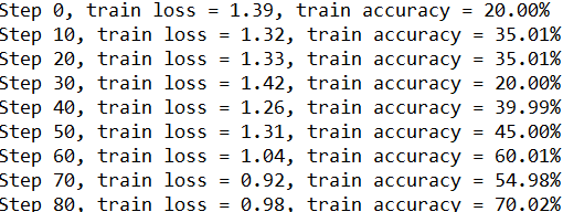
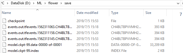
同时,训练结束后,在电脑指定的训练模型存储路径可看到保存的训练好的模型数据。
执行test模块,结果如下:
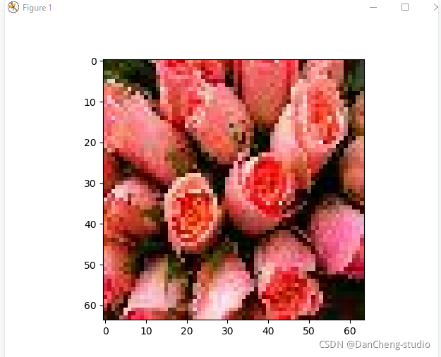
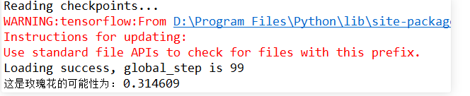
关闭显示的测试图片后,console查看测试结果如下:
做一个GUI交互界面

6 最后
🧿 更多资料, 项目分享:
https://gitee.com/dancheng-senior/postgraduate
这篇关于软著项目推荐 深度学习卷积神经网络的花卉识别的文章就介绍到这儿,希望我们推荐的文章对编程师们有所帮助!


