【Noise-Label】《Learning from Noisy Labels with Deep Neural Networks》

arXiv-2014

---

---

1 Background and Motivation

CNN 在分类任务上很不错！

However, this achievement is only possible because of large amount of labeled images.

大量的无误的 label 的获取 is a laborious task and takes a lot of time and money.

Our goal is to study the effect label noise on deep networks, and explore simple ways of improvement.

2 Advantages

提出了两种解决方法，然后确实 can improve state-of-the-art recognition models

3 Innovations

• propose several simple approaches to training deep neural networks on data with noisy labels

4 Method

• bottom-up model：在 base model 上 add additional noisy layer，为了 better match to noisy labels
• top-down model ：修改 noisy labels，然后再丢入 base model

4.1 Bottom-up Noise Model

noisy layer 即为 Q，定义如下：


Q 是一个 probability matrix，每项都是 positive，each column sums to one，因为是条件概率，比如有猫、狗、老鼠三类，$y^{\ast }$为老鼠，$y^{\ast }$ 转化为猫、狗、老鼠的概率和应该为 1！

用公式表示即为

• $\tilde{y}$：noisy label
• $y^{\ast }$：ground truth
• $\tilde{D}$：noisy distribution
  

确认了这种 motivation，……，网络学出来 $y^{\ast }$，通过 $Q$ 来 better match to the noisy labels，也即 $\tilde{y}$

没有 noisy label 的时候，可以设置 $Q$ 为 identity matrix，有 noisy label 后 $Q$ 通过 learning 学到，is linear，可以 backpropagation

加了 noisy layer 后，问题转化为求下面的式子，也即最大化释然估计！更细节的分析可以参考 【Noise-Label】《Training a Neural Network Based on Unreliable Human Annotation of Medical Images》

4.2 Estimating Noise Distribution Using Clean Data

matrix Q 是 classes 行 classes 列的，当类别很多的时候，很难用 cross-validation 的方法来估计，那么如何求解呢？
作者的方法，用 clean data $D^{\ast }$ 训练出来的模型算一个 confusion matrix，然后用 noisy data $\tilde{D}$ 训练出来的模型算一个 confusion matrix（confusion matrix 可以参考 【Keras-CNN】CIFAR-10 中的 2.7 小节，显示混淆矩阵），两者的差值 should be the noise distribution Q.

有点懵？这样可以吗？答案是可以的
误差来自于下面两个方面

• model mistakes
• noisy label mistakes

model mistakes 在 clean data 和 noisy data 训练出来的模型中都存在，difference 以后抵消了，然而，第二项 noisy label mistakes 仅 noisy data 训练出来的模型中存在！真是妙哉！！！

下面用公式来规范表示下上述作者的解法，The goal is to estimate the noise distribution of $\tilde{D}$

• M：pre-trained model，应该区分 $D^{\ast }$ 和 $\tilde{D}$ 的
• $D^{\ast }$：clean / clear data
• $\tilde{D}$：noisy data
• $C^{\ast }$：$D^{\ast }$ 在预训练模型 M 下训练出来的模型的 confusion matrix
• $\tilde{C}$：$\tilde{D}$ 在预训练模型 M 下训练出来的模型的 confusion matrix
• $j$：模型预测出来的类别，$i$ 表示真正的类别
• $c_{ij}^{\ast }$：$D^{\ast }$ 中 第 $j$ 类转化为 第 $i$ 类的概率
• ${\tilde{c}}_{ij}$：$\tilde{D}$ 中 第 $j$ 类转化为 第 $i$ 类的概率

其中 $c_{ij}^{\ast }$ 和 ${\tilde{c}}_{ij}$ 的关系如下：

• $r_{ij}$ denotes $p\left(y^{\ast }=i|\tilde{y}=j\right)$

用 matrix form 如下：

然后用 Bayes’ rule ，把 $r_{ij}$ 转化为 $q_{ji}$

$r_{ij}$ 通过 confusion matrix 的 difference 可以求出，$p(\tilde{y}=j)$ 可以通过标签求出，未知变量 $q_{ji}$ 和 $p(y\ast =i)$，一个方程，两个变量无穷解，好在之前有个约束，${\sum }_j{q}_{ji}=1$，这样两个方程两个解，可以求出我们需要的 $q_{ji}$ 了

对于上面形式的 R 的求法，作者说出了其弊端，

也即，如果 $R$ 和 $\tilde{C}$ 的相关性比较小，那么求逆的操作会放大存在的噪声！

作者用如下的形式来求 $R$，通过 L1 正则化，来加入 sparsity prior on R

加这种稀疏的先验也是有道理的，因为现实中的数据 are likely only be mislabeled with small set of other classes（医学图像处理领域就不好说咯，标注成本很高，很耗时）

求出了 $R$，就可以根据 Baye’s rule 来求 Noisy Distribution Q 了！

4.3 Learning Noise Distribution From Noisy Data

现实生活中，我们基本不可能有 100% clear data，这样的情况下，如何来评估 noisy distribution Q 呢？
我们用 noisy data 求出来的 noise distribution 为 $\hat{Q}$，用 clean data 求出来的为 $Q$，两者关系如下
$$\hat{Q}C=Q$$
$\hat{Q},C,Q$ both probability matrix

作者证明，求 minimize $tr(\hat{Q})$ 的最优解，满足 $\hat{Q}=Q$

矩阵A的迹（用 tr(A) 表示）就等于A的特征值的总和，也即矩阵A的主对角线元素的总和！In practice，作者 $tr(\hat{Q})$ 落地方式为对 $\hat{Q}$ 进行 weight decay 约束！（很想看看 code）

这里意思是，约束 tr($\hat{Q}$) 来使得 $\hat{Q}$ 更好的逼近 $Q$，作者证明了约束 tr($\hat{Q}$) 会使得 $\hat{Q}$ 向 $Q$ 靠拢，最优解就是 C 为 identity！

4.4 Training a Bottom-up Model

4.4.1 Noisy labels only

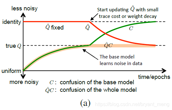
这个图是比较晦涩难懂的！也就是承接 4.3 小节的分析！

• 红色的线是 $\hat{Q}$ 随着 epoch 变化的情况，初始化为 identity
• 绿色的线是 $C$ 随着 epoch 变化的情况，初始化为 uniform
• 很粗的橘色线是 $\hat{Q}C$ 变化的情况

一开始固定 $\hat{Q}$ 为 identity，也就相当于不加 noisy layer 层，
训练到一定的阶段（validation error stops decreasing），来训练 weight decay 的 $\hat{Q}$ （开始训练 noisy layer 层）使得 $\hat{Q}$ 向真实的 $Q$ 逼近，使得 $C$ 向 identity 逼近，这样结果能进一步提升！
最后，validation error 不降的时候停止，防止 over-fitting

最后的结果

• $\hat{Q}$ 逼近于 $Q$
• $\hat{Q}C$ 逼近于 $Q$
• $C$ 逼近于 identity

如果测试 clean data 的时候，我们要 remove $\hat{Q}$ 或者设置为 $I$，但是验证 noisy label 的时候，还是需要加上 learned $\hat{Q}$！

4.4.2 Noisy and clean data

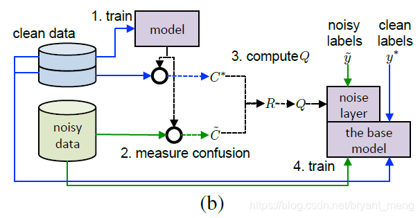
根据 4.2 节的分析，我们可以很容易的看懂这张图，

• 第一步，用 clear data 和 noisy data 分别 train 出来一个 model
• 第二步，计算两个模型的 confusion matrix $\tilde{C}$ 和 $C^{\ast }$
• 第三步，上一步的结果进行 difference，结果为 R，然后通过 Baye’s rule 进行转换，求出 Q
• 第四步，用学习到的 Q，作为 noisy layer，fix parameters，可以训练新的模型，noisy layer 之前，model 学到的是 $y\ast$，noisy layer 学到的是 $\tilde{y}$！！！

4.5 Top-down Noise Model

不是改变模型去拟合 noisy label，而是改变 noisy label，Given a noisy label is $i$, we replace it with vector label $s_i$

S be the conversion matrix consisting from column vectors $s_i$

1）Bottom-up Noise Model 的对数最大似然

2）Top-down Noise Model 的对数最大似然

• K is the number of classes

不能直接求 S（原因参考原文）作者用如$\alpha \cdot I+(1-\alpha )/K$ 的形式来处理，也即 label smoothing！（参考【Inception-v3】《Rethinking the Inception Architecture for Computer Vision》）

4.6 Reweighting of Noisy Data

降低 noisy data 的 weight，来结合 clear data 和 noisy data，这种方式在两种模型中都可以使用

• $N_c$：the number of clean data
• $N_n$：the number of noisy data
• $\gamma$：系数，超参数

5 Experiments

实验两个思路展开
一个是在 clean data 的数据集下，人为加噪声来评估 bottom-up（clean、noisy版）和 top-down 两种结构（5.2 小节）
二是在 noisy data 的数据下，也即不晓得 noisy distribution（5.3 小节）

5.1 Datasets

1）SVHN（32x32 images，600k for training，26k for testing）

2）CIFAR-10

all data are clean

3）CIFAR-10 with Tiny Images dataset

4）ImageNet with noisy images download from web search engines
其中1.3 M clean，1.4 noisy images 根据关键字在网上搜索，剔除掉和 imagenet 重合的部分！！！

5.2 Deliberate Label Noise

5.2.1 SVHN noisy only

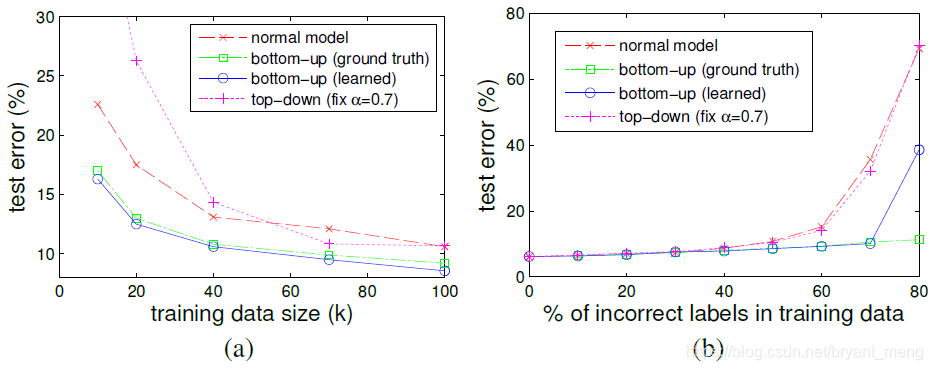
• （a）、（b）从不同的 training size 和 percentage of incorrect labels 两个角度来观测 test error！（a）50%，（b）100k
• bottom-up 结果总比 normal model 好，top-down 不尽人意
• bottom-up（ground truth）表示Q用gt的 noisy distribution，因为 SVHN 是干净的数据，噪声是自己加的，所以知道 noisy distribution
• 训练 bottom-up（learned）的时候，前 5 个 epoch fixed，后100个 learned，weight decay 0.05
• bottom-up（gt） 和（learned）55开，说明作者的这种 idea 是 work 的，下面的图很好说明（estimated $\hat{Q}$ 的介绍请看 5.2.3 小节）

下面一个图尽显 bottom-up 模型的优势（颜色越深，error 越高）

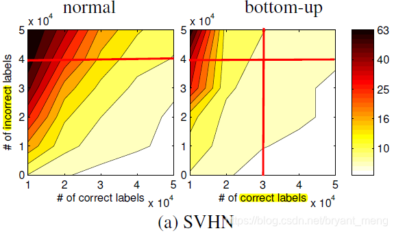
从我画的红线中可以看出，

• correct 50k 和 incorrect 40k 时（两条横线），明显 bottom-up 好
• bottom-up 在 correct 30k 和 incorrect 50k 时，能达到 normal correct 50k 和 incorrect 40k 同样的正确率！

5.2.2 CIFAR-10 noisy only

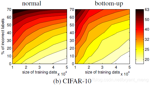
前 50 epoch fixed $\hat{Q}$，后 70 epoch update $\hat{Q}$，weight decay 0.05 or 1

5.2.3 CIFAR-10 clean + noisy

20 k clean data estimate Q
30 k noisy data 来 train final model

1）用 20 k 中的 10 k clean data 来 train 一个 model，30% test error，这就是 model mistakes
2）在 model 上，用 剩下的 10 k clean data 和 30 k noisy data 来算 two confusion matrix，difference 以后的结果为 R，然后计算出Q，名为 estimate $\hat{Q}$，下图的 estimate $\hat{Q}$ 有50%的噪声，estimate $\hat{Q}$ 和 true Q 相差不是很大！说明这个方法的可行性！

3）用 estimated $\hat{Q}$ 就可以来 train 带有 noisy label 的 data 了！

这个表可以看出，estimated 这种方式最 work，true Q 和 estimate $\hat{Q}$ 都是 fixed parameters 来 trained new model 的！！！

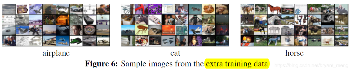
5.3 CIFAR-10 + Tiny Images

CIFAR-10 was originally created by cleaning up a subset of Tiny Images

• 50 k from CIFAR-10
• 150 k noisy data from excluded set of Tiny Images

• bottom-up model：前 50 epoch fixed $\hat{Q}$，后 epoch update $\hat{Q}$ with no weight decay
• top-down model：$\alpha =0.5$

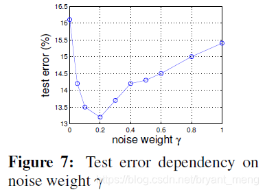
两种模型结合，$\gamma =0.2$ 时效果最好！给 noisy label 加权，看下效果

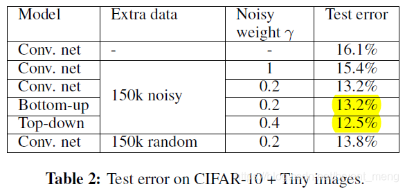
第四列对应着 figure 7，可以看出 bottom up 的效果一般，top-down 反而好，作者给出的解释是，因为 extra data 中有太多的非 10类的图片，violate the noise model ，而 top-down 表现好的原因是 impose a more uniform label distribution on these outside images！！！

作者用最后一列的实验来验证了他上述的 hypothesis，150k random 的label 为 uniform label，相当于 $\alpha =0.1$，里面 not just the excluded set（Tiny Images），效果确实不错！如下是作者对 $\alpha =0.1$ 的总结！！！

5.4 ImageNet + Web Image Search

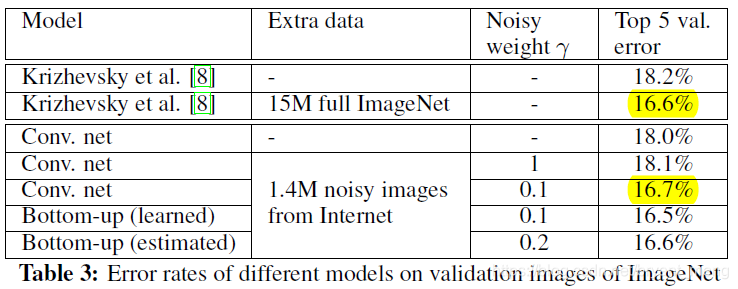
作者应该只用 1.5 M 的clean data来 train model，然后 extra data 是配合 clean data 一起训练的

• 从 第三行和第四行看出，联合 data train 并不能提高 performance，相对只 train clean data
• 从 四五行可以看出，改变 noisy data 的权重，升了 1.4 个点，厉害
• 从黄色的部分可以看出，1.4 M noisy data 加权的效果和 15 M full ImageNet 的相仿，amazing

This demonstrates that noisy data can be very beneficial for training.

6 Conclusion（own）

• bottom-up（clean，noisy 版）
• top-down（label smoothing 5.3小节）
• reweighting of Noisy Data（提升明显，5.4小节）

bottom-up clean 版（手头有100%的clean data）

bottom-up noisy版（手头的数据不干净，weight decay on Q）