Coursera | Mathematics for Machine Learning 专项课程

本文主要是介绍Coursera | Mathematics for Machine Learning 专项课程 | Linear Algebra，希望对大家解决编程问题提供一定的参考价值，需要的开发者们随着小编来一起学习吧！

本文为学习笔记，记录了由Imperial College London推出的Coursera专项课程——Mathematics for Machine Learning中Course One: Mathematics for Machine Learning: Linear Algebra中全部Programming Assignment代码，均已通过测试，得分均为10/10。

Identifying special matrices

Instructions

Matrices in Python

Test your code before submission

Gram-Schmidt process

Instructions

Matrices in Python

Test your code before submission

Reflecting Bear

Background

Instructions

Matrices in Python

Test your code before submission

PageRank

Part 1 - Worksheet

Introduction

PageRank as a linear algebra problem

Damping Parameter

Part 2 - Assessment

Test your code before submission

Identifying special matrices

Instructions

In this assignment, you shall write a function that will test if a 4×4 matrix is singular, i.e. to determine if an inverse exists, before calculating it.

You shall use the method of converting a matrix to echelon form, and testing if this fails by leaving zeros that can’t be removed on the leading diagonal.

Don't worry if you've not coded before, a framework for the function has already been written. Look through the code, and you'll be instructed where to make changes. We'll do the first two rows, and you can use this as a guide to do the last two.

Matrices in Python

In the numpy package in Python, matrices are indexed using zero for the top-most column and left-most row. I.e., the matrix structure looks like this:

A[0, 0]  A[0, 1]  A[0, 2]  A[0, 3]
A[1, 0]  A[1, 1]  A[1, 2]  A[1, 3]
A[2, 0]  A[2, 1]  A[2, 2]  A[2, 3]
A[3, 0]  A[3, 1]  A[3, 2]  A[3, 3]

You can access the value of each element individually using,

A[n, m]

which will give the n'th row and m'th column (starting with zero). You can also access a whole row at a time using,

A[n]

Which you will see will be useful when calculating linear combinations of rows.

A final note - Python is sensitive to indentation. All the code you should complete will be at the same level of indentation as the instruction comment.

# GRADED FUNCTION
import numpy as np# Our function will go through the matrix replacing each row in order turning it into echelon form.
# If at any point it fails because it can't put a 1 in the leading diagonal,
# we will return the value True, otherwise, we will return False.
# There is no need to edit this function.
def isSingular(A) :B = np.array(A, dtype=np.float_) # Make B as a copy of A, since we're going to alter it's values.try:fixRowZero(B)fixRowOne(B)fixRowTwo(B)fixRowThree(B)except MatrixIsSingular:return Truereturn False# This next line defines our error flag. For when things go wrong if the matrix is singular.
# There is no need to edit this line.
class MatrixIsSingular(Exception): pass# For Row Zero, all we require is the first element is equal to 1.
# We'll divide the row by the value of A[0, 0].
# This will get us in trouble though if A[0, 0] equals 0, so first we'll test for that,
# and if this is true, we'll add one of the lower rows to the first one before the division.
# We'll repeat the test going down each lower row until we can do the division.
# There is no need to edit this function.
def fixRowZero(A) :if A[0,0] == 0 :A[0] = A[0] + A[1]if A[0,0] == 0 :A[0] = A[0] + A[2]if A[0,0] == 0 :A[0] = A[0] + A[3]if A[0,0] == 0 :raise MatrixIsSingular()A[0] = A[0] / A[0,0]return A# First we'll set the sub-diagonal elements to zero, i.e. A[1,0].
# Next we want the diagonal element to be equal to one.
# We'll divide the row by the value of A[1, 1].
# Again, we need to test if this is zero.
# If so, we'll add a lower row and repeat setting the sub-diagonal elements to zero.
# There is no need to edit this function.
def fixRowOne(A) :A[1] = A[1] - A[1,0] * A[0]if A[1,1] == 0 :A[1] = A[1] + A[2]A[1] = A[1] - A[1,0] * A[0]if A[1,1] == 0 :A[1] = A[1] + A[3]A[1] = A[1] - A[1,0] * A[0]if A[1,1] == 0 :raise MatrixIsSingular()A[1] = A[1] / A[1,1]return A# This is the first function that you should complete.
# Follow the instructions inside the function at each comment.
def fixRowTwo(A) :# Insert code below to set the sub-diagonal elements of row two to zero (there are two of them).A[2] = A[2] - A[0] * A[2, 0]A[2] = A[2] - A[1] * A[2, 1]# Next we'll test that the diagonal element is not zero.if A[2,2] == 0 :# Insert code below that adds a lower row to row 2.A[2] = A[2] + A[3]# Now repeat your code which sets the sub-diagonal elements to zero.A[2] = A[2] - A[0] * A[2, 0]A[2] = A[2] - A[1] * A[2, 1]if A[2,2] == 0 :raise MatrixIsSingular()# Finally set the diagonal element to one by dividing the whole row by that element.A[2] = A[2] / A[2, 2]return A# You should also complete this function
# Follow the instructions inside the function at each comment.
def fixRowThree(A) :# Insert code below to set the sub-diagonal elements of row three to zero.A[3] = A[3] - A[0] * A[3, 0]A[3] = A[3] - A[1] * A[3, 1]A[3] = A[3] - A[2] * A[3, 2]# Complete the if statement to test if the diagonal element is zero.if A[3, 3] == 0:raise MatrixIsSingular()# Transform the row to set the diagonal element to one.A[3] = A[3] / A[3, 3]return A

Test your code before submission

To test the code you've written above, run the cell (select the cell above, then press the play button [ ▶| ] or press shift-enter). You can then use the code below to test out your function. You don't need to submit this cell; you can edit and run it as much as you like.

Try out your code on tricky test cases!

A = np.array([[2, 0, 0, 0],[0, 3, 0, 0],[0, 0, 4, 4],[0, 0, 5, 5]], dtype=np.float_)
isSingular(A)

运行结果：

True

A = np.array([[0, 7, -5, 3],[2, 8, 0, 4],[3, 12, 0, 5],[1, 3, 1, 3]], dtype=np.float_)
fixRowZero(A)

运行结果：

array([[  1. ,   7.5,  -2.5,   3.5],[  2. ,   8. ,   0. ,   4. ],[  3. ,  12. ,   0. ,   5. ],[  1. ,   3. ,   1. ,   3. ]])

fixRowOne(A)

运行结果：

array([[  1.        ,   7.5       ,  -2.5       ,   3.5       ],[ -0.        ,   1.        ,  -0.71428571,   0.42857143],[  3.        ,  12.        ,   0.        ,   5.        ],[  1.        ,   3.        ,   1.        ,   3.        ]])

fixRowTwo(A)

运行结果：

array([[ 1.        ,  7.5       , -2.5       ,  3.5       ],[-0.        ,  1.        , -0.71428571,  0.42857143],[ 0.        ,  0.        ,  1.        ,  1.5       ],[ 1.        ,  3.        ,  1.        ,  3.        ]])

fixRowThree(A)

运行结果：

array([[ 1.        ,  7.5       , -2.5       ,  3.5       ],[-0.        ,  1.        , -0.71428571,  0.42857143],[ 0.        ,  0.        ,  1.        ,  1.5       ],[ 0.        ,  0.        ,  0.        ,  1.        ]])

Gram-Schmidt process

Instructions

In this assignment you will write a function to perform the Gram-Schmidt procedure, which takes a list of vectors and forms an orthonormal basis from this set. As a corollary, the procedure allows us to determine the dimension of the space spanned by the basis vectors, which is equal to or less than the space which the vectors sit.

You'll start by completing a function for 4 basis vectors, before generalising to when an arbitrary number of vectors are given.

Again, a framework for the function has already been written. Look through the code, and you'll be instructed where to make changes. We'll do the first two rows, and you can use this as a guide to do the last two.

Matrices in Python

Remember the structure for matrices in numpy is,

A[0, 0]  A[0, 1]  A[0, 2]  A[0, 3]
A[1, 0]  A[1, 1]  A[1, 2]  A[1, 3]
A[2, 0]  A[2, 1]  A[2, 2]  A[2, 3]
A[3, 0]  A[3, 1]  A[3, 2]  A[3, 3]

You can access the value of each element individually using,

A[n, m]

You can also access a whole row at a time using,

A[n]

Building on last assignment, in this exercise you will need to select whole columns at a time. This can be done with,

A[:, m]

which will select the m'th column (starting at zero).

In this exercise, you will need to take the dot product between vectors. This can be done using the @ operator. To dot product vectors u and v, use the code,

u @ v

All the code you should complete will be at the same level of indentation as the instruction comment.

# GRADED FUNCTION
import numpy as np
import numpy.linalg as laverySmallNumber = 1e-14 # That's 1×10⁻¹⁴ = 0.00000000000001# Our first function will perform the Gram-Schmidt procedure for 4 basis vectors.
# We'll take this list of vectors as the columns of a matrix, A.
# We'll then go through the vectors one at a time and set them to be orthogonal
# to all the vectors that came before it. Before normalising.
# Follow the instructions inside the function at each comment.
# You will be told where to add code to complete the function.
def gsBasis4(A) :B = np.array(A, dtype=np.float_) # Make B as a copy of A, since we're going to alter it's values.# The zeroth column is easy, since it has no other vectors to make it normal to.# All that needs to be done is to normalise it. I.e. divide by its modulus, or norm.B[:, 0] = B[:, 0] / la.norm(B[:, 0])# For the first column, we need to subtract any overlap with our new zeroth vector.B[:, 1] = B[:, 1] - B[:, 1] @ B[:, 0] * B[:, 0]# If there's anything left after that subtraction, then B[:, 1] is linearly independant of B[:, 0]# If this is the case, we can normalise it. Otherwise we'll set that vector to zero.if la.norm(B[:, 1]) > verySmallNumber :B[:, 1] = B[:, 1] / la.norm(B[:, 1])else :B[:, 1] = np.zeros_like(B[:, 1])# Now we need to repeat the process for column 2.# Insert two lines of code, the first to subtract the overlap with the zeroth vector,# and the second to subtract the overlap with the first.B[:, 2] = B[:, 2] - B[:, 2] @ B[:, 0] * B[:, 0]B[:, 2] = B[:, 2] - B[:, 2] @ B[:, 1] * B[:, 1]# Again we'll need to normalise our new vector.# Copy and adapt the normalisation fragment from above to column 2.if la.norm(B[:, 2]) > verySmallNumber:B[:, 2] = B[:, 2] / la.norm(B[:, 2])else:B[:, 2] = np.zeros_like(B[:, 2])# Finally, column three:# Insert code to subtract the overlap with the first three vectors.B[:, 3] = B[:, 3] - B[:, 3] @ B[:, 0] * B[:, 0]B[:, 3] = B[:, 3] - B[:, 3] @ B[:, 1] * B[:, 1]B[:, 3] = B[:, 3] - B[:, 3] @ B[:, 2] * B[:, 2]# Now normalise if possibleif la.norm(B[:, 3]) > verySmallNumber:B[:, 3] = B[:, 3] / la.norm(B[:, 3])else:B[:, 3] = np.zeros_like(B[:, 3])# Finally, we return the result:return B# The second part of this exercise will generalise the procedure.
# Previously, we could only have four vectors, and there was a lot of repeating in the code.
# We'll use a for-loop here to iterate the process for each vector.
def gsBasis(A) :B = np.array(A, dtype=np.float_) # Make B as a copy of A, since we're going to alter it's values.# Loop over all vectors, starting with zero, label them with ifor i in range(B.shape[1]) :# Inside that loop, loop over all previous vectors, j, to subtract.for j in range(i) :# Complete the code to subtract the overlap with previous vectors.# you'll need the current vector B[:, i] and a previous vector B[:, j]B[:, i] = B[:, i] - B[:, i] @ B[:, j] * B[:, j]# Next insert code to do the normalisation test for B[:, i]if la.norm(B[:, i]) > verySmallNumber:B[:, i] = B[:, i] / la.norm(B[:, i])else:B[:, i] = np.zeros_like(B[:, i])# Finally, we return the result:return B# This function uses the Gram-schmidt process to calculate the dimension
# spanned by a list of vectors.
# Since each vector is normalised to one, or is zero,
# the sum of all the norms will be the dimension.
def dimensions(A) :return np.sum(la.norm(gsBasis(A), axis=0))

Test your code before submission

Try out your code on tricky test cases!

V = np.array([[1,0,2,6],[0,1,8,2],[2,8,3,1],[1,-6,2,3]], dtype=np.float_)
gsBasis4(V)

运行结果：

array([[ 0.40824829, -0.1814885 ,  0.04982278,  0.89325973],[ 0.        ,  0.1088931 ,  0.99349591, -0.03328918],[ 0.81649658,  0.50816781, -0.06462163, -0.26631346],[ 0.40824829, -0.83484711,  0.07942048, -0.36063281]])

# Once you've done Gram-Schmidt once,
# doing it again should give you the same result. Test this:
U = gsBasis4(V)
gsBasis4(U)

运行结果：

array([[ 0.40824829, -0.1814885 ,  0.04982278,  0.89325973],[ 0.        ,  0.1088931 ,  0.99349591, -0.03328918],[ 0.81649658,  0.50816781, -0.06462163, -0.26631346],[ 0.40824829, -0.83484711,  0.07942048, -0.36063281]])

# Try the general function too.
gsBasis(V)

运行结果：

array([[ 0.40824829, -0.1814885 ,  0.04982278,  0.89325973],[ 0.        ,  0.1088931 ,  0.99349591, -0.03328918],[ 0.81649658,  0.50816781, -0.06462163, -0.26631346],[ 0.40824829, -0.83484711,  0.07942048, -0.36063281]])

# See what happens for non-square matrices
A = np.array([[3,2,3],[2,5,-1],[2,4,8],[12,2,1]], dtype=np.float_)
gsBasis(A)

运行结果：

array([[ 0.23643312,  0.18771349,  0.22132104],[ 0.15762208,  0.74769023, -0.64395812],[ 0.15762208,  0.57790444,  0.72904263],[ 0.94573249, -0.26786082, -0.06951101]])

dimensions(A)

运行结果：

3.0

B = np.array([[6,2,1,7,5],[2,8,5,-4,1],[1,-6,3,2,8]], dtype=np.float_)
gsBasis(B)

运行结果：

array([[ 0.93704257, -0.12700832, -0.32530002,  0.        ,  0.        ],[ 0.31234752,  0.72140727,  0.61807005,  0.        ,  0.        ],[ 0.15617376, -0.6807646 ,  0.71566005,  0.        ,  0.        ]])

dimensions(B)

运行结果：

3.0

# Now let's see what happens when we have one vector that is a linear combination of the others.
C = np.array([[1,0,2],[0,1,-3],[1,0,2]], dtype=np.float_)
gsBasis(C)

运行结果：

array([[ 0.70710678,  0.        ,  0.        ],[ 0.        ,  1.        ,  0.        ],[ 0.70710678,  0.        ,  0.        ]])

dimensions(C)

运行结果：

2.0

Reflecting Bear

Background

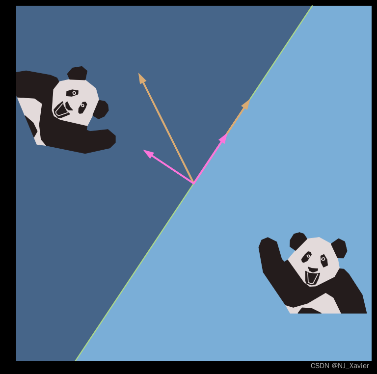
Panda Bear is confused. He is trying to work out how things should look when reflected in a mirror, but is getting the wrong results. In Bear's coordinates, the mirror lies along the first axis. But, as is the way with bears, his coordinate system is not orthonormal: so what he thinks is the direction perpendicular to the mirror isn't actually the direction the mirror reflects in. Help Bear write a code that will do his matrix calculations properly!

Instructions

In this assignment you will write a Python function that will produce a transformation matrix for reflecting vectors in an arbitrarily angled mirror.

Building on the last assingment, where you wrote a code to construct an orthonormal basis that spans a set of input vectors, here you will take a matrix which takes simple form in that basis, and transform it into our starting basis. Recall the from the last video,

$T = ET_EE^{-1}$

You will write a function that will construct this matrix. This assessment is not conceptually complicated, but will build and test your ability to express mathematical ideas in code. As such, your final code submission will be relatively short, but you will receive less structure on how to write it.

Matrices in Python

For this exercise, we shall make use of the @ operator again. Recall from the last exercise, we used this operator to take the dot product of vectors. In general the operator will combine vectors and/or matrices in the expected linear algebra way, i.e. it will be either the vector dot product, matrix multiplication, or matrix operation on a vector, depending on it's input. For example to calculate the following expressions,

$a=s \cdot t$

$s = At$

$M = AB$ ,

One would use the code,

a = s @ t
s = A @ t
M = A @ B

(This is in contrast to the ∗ operator, which performs element-wise multiplication, or multiplication by a scalar.)

You may need to use some of the following functions:

inv(A)
transpose(A)
gsBasis(A)

These, respectively, take the inverse of a matrix, give the transpose of a matrix, and produce a matrix of orthonormal column vectors given a general matrix of column vectors - i.e. perform the Gram-Schmidt process. This exercise will require you to combine some of these functions.

# PACKAGE
# Run this cell first once to load the dependancies.
import numpy as np
from numpy.linalg import norm, inv
from numpy import transpose
from readonly.bearNecessities import *

# GRADED FUNCTION
# You should edit this cell.# In this function, you will return the transformation matrix T,
# having built it out of an orthonormal basis set E that you create from Bear's Basis
# and a transformation matrix in the mirror's coordinates TE.
def build_reflection_matrix(bearBasis) : # The parameter bearBasis is a 2×2 matrix that is passed to the function.# Use the gsBasis function on bearBasis to get the mirror's orthonormal basis.E = gsBasis(bearBasis)# Write a matrix in component form that performs the mirror's reflection in the mirror's basis.# Recall, the mirror operates by negating the last component of a vector.# Replace a,b,c,d with appropriate valuesTE = np.array([[1, 0],[0, -1]])# Combine the matrices E and TE to produce your transformation matrix.T = E @ TE @ transpose(E)# Finally, we return the result. There is no need to change this line.return T

Test your code before submission

The code below will show a picture of Panda Bear. If you have correctly implemented the function above, you will also see Bear's reflection in his mirror. The orange axes are Bear's basis, and the pink axes are the mirror's orthonormal basis.

# First load Pyplot, a graph plotting library.
%matplotlib inline
import matplotlib.pyplot as plt# This is the matrix of Bear's basis vectors.
# (When you've done the exercise once, see what happns when you change Bear's basis.)
bearBasis = np.array([[1,   -1],[1.5, 2]])
# This line uses your code to build a transformation matrix for us to use.
T = build_reflection_matrix(bearBasis)# Bear is drawn as a set of polygons, the vertices of which are placed as a matrix list of column vectors.
# We have three of these non-square matrix lists: bear_white_fur, bear_black_fur, and bear_face.
# We'll make new lists of vertices by applying the T matrix you've calculated.
reflected_bear_white_fur = T @ bear_white_fur
reflected_bear_black_fur = T @ bear_black_fur
reflected_bear_face = T @ bear_face# This next line runs a code to set up the graphics environment.
ax = draw_mirror(bearBasis)# We'll first plot Bear, his white fur, his black fur, and his face.
ax.fill(bear_white_fur[0], bear_white_fur[1], color=bear_white, zorder=1)
ax.fill(bear_black_fur[0], bear_black_fur[1], color=bear_black, zorder=2)
ax.plot(bear_face[0], bear_face[1], color=bear_white, zorder=3)# Next we'll plot Bear's reflection.
ax.fill(reflected_bear_white_fur[0], reflected_bear_white_fur[1], color=bear_white, zorder=1)
ax.fill(reflected_bear_black_fur[0], reflected_bear_black_fur[1], color=bear_black, zorder=2)
ax.plot(reflected_bear_face[0], reflected_bear_face[1], color=bear_white, zorder=3);

运行结果：

PageRank

In this notebook, you'll build on your knowledge of eigenvectors and eigenvalues by exploring the PageRank algorithm. The notebook is in two parts, the first is a worksheet to get you up to speed with how the algorithm works - here we will look at a micro-internet with fewer than 10 websites and see what it does and what can go wrong. The second is an assessment which will test your application of eigentheory to this problem by writing code and calculating the page rank of a large network representing a sub-section of the internet.

Part 1 - Worksheet

Introduction

PageRank (developed by Larry Page and Sergey Brin) revolutionized web search by generating a ranked list of web pages based on the underlying connectivity of the web. The PageRank algorithm is based on an ideal random web surfer who, when reaching a page, goes to the next page by clicking on a link. The surfer has equal probability of clicking any link on the page and, when reaching a page with no links, has equal probability of moving to any other page by typing in its URL. In addition, the surfer may occasionally choose to type in a random URL instead of following the links on a page. The PageRank is the ranked order of the pages from the most to the least probable page the surfer will be viewing.

# Before we begin, let's load the libraries.
%pylab notebook
import numpy as np
import numpy.linalg as la
from readonly.PageRankFunctions import *
np.set_printoptions(suppress=True)

PageRank as a linear algebra problem

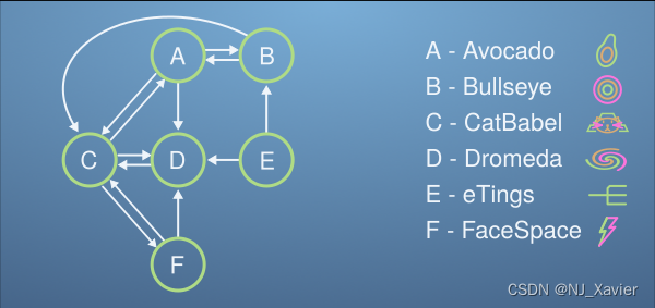
Let's imagine a micro-internet, with just 6 websites (Avocado, Bullseye, CatBabel, Dromeda, eTings, and FaceSpace). Each website links to some of the others, and this forms a network as shown,

The design principle of PageRank is that important websites will be linked to by important websites. This somewhat recursive principle will form the basis of our thinking.

Imagine we have 100 Procrastinating Pats on our micro-internet, each viewing a single website at a time. Each minute the Pats follow a link on their website to another site on the micro-internet. After a while, the websites that are most linked to will have more Pats visiting them, and in the long run, each minute for every Pat that leaves a website, another will enter keeping the total numbers of Pats on each website constant. The PageRank is simply the ranking of websites by how many Pats they have on them at the end of this process.

We represent the number of Pats on each website with the vector,

$r = \begin{bmatrix} r_A \\ r_B \\ r_C \\ r_D \\ r_E \\ r_F \\ \end{bmatrix}$

And say that the number of Pats on each website in minute $i +1$ is related to those at minute $i$ by the matrix transformation

$r^{(i+1)} = Lr^{(i)}$

with the matrix $L$ taking the form,

$\begin{bmatrix} L_{A{\rightarrow}A} & L_{B{\rightarrow}A} & L_{C{\rightarrow}A} & L_{D{\rightarrow}A} & L_{E{\rightarrow}A} & L_{F{\rightarrow}A}\\ L_{A{\rightarrow}B} & L_{B{\rightarrow}B} & L_{C{\rightarrow}B} & L_{D{\rightarrow}B} & L_{E{\rightarrow}B} & L_{F{\rightarrow}B}\\ L_{A{\rightarrow}C} & L_{B{\rightarrow}C} & L_{C{\rightarrow}C} & L_{D{\rightarrow}C} & L_{E{\rightarrow}C} & L_{F{\rightarrow}C}\\ L_{A{\rightarrow}D} & L_{B{\rightarrow}D} & L_{C{\rightarrow}D} & L_{D{\rightarrow}D} & L_{E{\rightarrow}D} & L_{F{\rightarrow}D}\\ L_{A{\rightarrow}E} & L_{B{\rightarrow}E} & L_{C{\rightarrow}E} & L_{D{\rightarrow}E} & L_{E{\rightarrow}E} & L_{F{\rightarrow}E}\\ L_{A{\rightarrow}F} & L_{B{\rightarrow}F} & L_{C{\rightarrow}F} & L_{D{\rightarrow}F} & L_{E{\rightarrow}F} & L_{F{\rightarrow}F} \end{bmatrix}$

where the columns represent the probability of leaving a website for any other website, and sum to one. The rows determine how likely you are to enter a website from any other, though these need not add to one. The long time behaviour of this system is when $r^{(i+1)} = r^{(i)}$ , so we'll drop the superscripts here, and that allows us to write,

$Lr = r$

which is an eigenvalue equation for the matrix $L$ , with eigenvalue 1 (this is guaranteed by the probabalistic structure of the matrix $L$ ).

Complete the matrix $L$ below, we've left out the column for which websites the FaceSpace website (F) links to. Remember, this is the probability to click on another website from this one, so each column should add to one (by scaling by the number of links).

# Replace the ??? here with the probability of clicking a link to each website when leaving Website F (FaceSpace).
L = np.array([[0,   1/2, 1/3, 0, 0,   0 ],[1/3, 0,   0,   0, 1/2, 0 ],[1/3, 1/2, 0,   1, 0,   1/2 ],[1/3, 0,   1/3, 0, 1/2, 1/2 ],[0,   0,   0,   0, 0,   0 ],[0,   0,   1/3, 0, 0,   0 ]])

In principle, we could use a linear algebra library, as below, to calculate the eigenvalues and vectors. And this would work for a small system. But this gets unmanagable for large systems. And since we only care about the principal eigenvector (the one with the largest eigenvalue, which will be 1 in this case), we can use the power iteration method which will scale better, and is faster for large systems.

Use the code below to peek at the PageRank for this micro-internet.

eVals, eVecs = la.eig(L) # Gets the eigenvalues and vectors
order = np.absolute(eVals).argsort()[::-1] # Orders them by their eigenvalues
eVals = eVals[order]
eVecs = eVecs[:,order]r = eVecs[:, 0] # Sets r to be the principal eigenvector
100 * np.real(r / np.sum(r)) # Make this eigenvector sum to one, then multiply by 100 Procrastinating Pats

运行结果：

array([ 16.        ,   5.33333333,  40.        ,  25.33333333,0.        ,  13.33333333])

We can see from this list, the number of Procrastinating Pats that we expect to find on each website after long times. Putting them in order of popularity (based on this metric), the PageRank of this micro-internet is:

CatBabel, Dromeda, Avocado, FaceSpace, Bullseye, eTings

Referring back to the micro-internet diagram, is this what you would have expected? Convince yourself that based on which pages seem important given which others link to them, that this is a sensible ranking.

Let's now try to get the same result using the Power-Iteration method that was covered in the video. This method will be much better at dealing with large systems.

First let's set up our initial vector, $r^{(0)}$ , so that we have our 100 Procrastinating Pats equally distributed on each of our 6 websites.

r = 100 * np.ones(6) / 6 # Sets up this vector (6 entries of 1/6 × 100 each)
r # Shows it's value

运行结果：

array([ 16.66666667,  16.66666667,  16.66666667,  16.66666667,16.66666667,  16.66666667])

Next, let's update the vector to the next minute, with the matrix $L$ . Run the following cell multiple times, until the answer stabilises.

r = L @ r # Apply matrix L to r
r # Show it's value
# Re-run this cell multiple times to converge to the correct answer.

运行结果：

array([ 13.88888889,  13.88888889,  38.88888889,  27.77777778,0.        ,   5.55555556])

We can automate applying this matrix multiple times as follows,

r = 100 * np.ones(6) / 6 # Sets up this vector (6 entries of 1/6 × 100 each)
for i in np.arange(100) : # Repeat 100 timesr = L @ r
r

运行结果：

array([ 16.        ,   5.33333333,  40.        ,  25.33333333,0.        ,  13.33333333])

Or even better, we can keep running until we get to the required tolerance.

r = 100 * np.ones(6) / 6 # Sets up this vector (6 entries of 1/6 × 100 each)
lastR = r
r = L @ r
i = 0
while la.norm(lastR - r) > 0.01 :lastR = rr = L @ ri += 1
print(str(i) + " iterations to convergence.")
r

运行结果：

18 iterations to convergence.

array([ 16.00149917,   5.33252025,  39.99916911,  25.3324738 ,0.        ,  13.33433767])

See how the PageRank order is established fairly quickly, and the vector converges on the value we calculated earlier after a few tens of repeats.

Congratulations! You've just calculated your first PageRank!

Damping Parameter

The system we just studied converged fairly quickly to the correct answer. Let's consider an extension to our micro-internet where things start to go wrong.

Say a new website is added to the micro-internet: Geoff's Website. This website is linked to by FaceSpace and only links to itself.

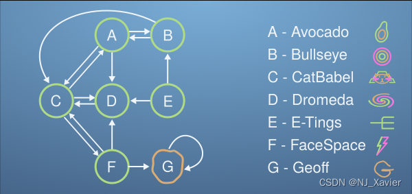
Intuitively, only FaceSpace, which is in the bottom half of the page rank, links to this website amongst the two others it links to, so we might expect Geoff's site to have a correspondingly low PageRank score.

Build the new LL matrix for the expanded micro-internet, and use Power-Iteration on the Procrastinating Pat vector. See what happens…

 # We'll call this one L2, to distinguish it from the previous L.
L2 = np.array([[0,   1/2, 1/3, 0, 0,   0, 0 ],[1/3, 0,   0,   0, 1/2, 0, 0 ],[1/3, 1/2, 0,   1, 0,   1/3, 0 ],[1/3, 0,   1/3, 0, 1/2, 1/3, 0 ],[0,   0,   0,   0, 0,   0, 0 ],[0,   0,   1/3, 0, 0,   0, 0 ],[0,   0,   0,   0, 0,   1/3, 1 ]])

r = 100 * np.ones(7) / 7 # Sets up this vector (6 entries of 1/6 × 100 each)
lastR = r
r = L2 @ r
i = 0
while la.norm(lastR - r) > 0.01 :lastR = rr = L2 @ ri += 1
print(str(i) + " iterations to convergence.")
r

运行结果：

131 iterations to convergence.

array([  0.03046998,   0.01064323,   0.07126612,   0.04423198,0.        ,   0.02489342,  99.81849527])

That's no good! Geoff seems to be taking all the traffic on the micro-internet, and somehow coming at the top of the PageRank. This behaviour can be understood, because once a Pat get's to Geoff's Website, they can't leave, as all links head back to Geoff.

To combat this, we can add a small probability that the Procrastinating Pats don't follow any link on a webpage, but instead visit a website on the micro-internet at random. We'll say the probability of them following a link is dd and the probability of choosing a random website is therefore $1 - d$ . We can use a new matrix to work out where the Pat's visit each minute.

$M = dL + \frac {1-d} n J$

where $J$ is an n×nn×n matrix where every element is one.

If $d$ is one, we have the case we had previously, whereas if $d$ is zero, we will always visit a random webpage and therefore all webpages will be equally likely and equally ranked. For this extension to work best, $1-d$ should be somewhat small - though we won't go into a discussion about exactly how small.

Let's retry this PageRank with this extension.

d = 0.5 # Feel free to play with this parameter after running the code once.
M = d * L2 + (1-d)/7 * np.ones([7, 7]) # np.ones() is the J matrix, with ones for each entry.

r = 100 * np.ones(7) / 7 # Sets up this vector (6 entries of 1/6 × 100 each)
lastR = r
r = M @ r
i = 0
while la.norm(lastR - r) > 0.01 :lastR = rr = M @ ri += 1
print(str(i) + " iterations to convergence.")
r

运行结果：

8 iterations to convergence.

array([ 13.68217054,  11.20902965,  22.41964343,  16.7593433 ,7.14285714,  10.87976354,  17.90719239])

This is certainly better, the PageRank gives sensible numbers for the Procrastinating Pats that end up on each webpage. This method still predicts Geoff has a high ranking webpage however. This could be seen as a consequence of using a small network. We could also get around the problem by not counting self-links when producing the L matrix (an if a website has no outgoing links, make it link to all websites equally). We won't look further down this route, as this is in the realm of improvements to PageRank, rather than eigenproblems.

You are now in a good position, having gained an understanding of PageRank, to produce your own code to calculate the PageRank of a website with thousands of entries.

Good Luck!

Part 2 - Assessment

In this assessment, you will be asked to produce a function that can calculate the PageRank for an arbitrarily large probability matrix. This, the final assignment of the course, will give less guidance than previous assessments. You will be expected to utilise code from earlier in the worksheet and re-purpose it to your needs.

# PACKAGE
# Here are the imports again, just in case you need them.
# There is no need to edit or submit this cell.
import numpy as np
import numpy.linalg as la
from readonly.PageRankFunctions import *
np.set_printoptions(suppress=True)

# GRADED FUNCTION
# Complete this function to provide the PageRank for an arbitrarily sized internet.
# I.e. the principal eigenvector of the damped system, using the power iteration method.
# (Normalisation doesn't matter here)
# The functions inputs are the linkMatrix, and d the damping parameter - as defined in this worksheet.
# (The damping parameter, d, will be set by the function - no need to set this yourself.)
def pageRank(linkMatrix, d) :n = linkMatrix.shape[0]M = d * linkMatrix + (1 - d) / n * np.ones([n, n])r = 100 * np.ones(n) / nlastR = rr = M @ ri = 0while la.norm(lastR - r) > 0.01 :lastR = rr = M @ ri += 1return r

Test your code before submission

# Use the following function to generate internets of different sizes.
generate_internet(5)

运行结果：

array([[ 1. ,  0. ,  0. ,  0. ,  0.2],[ 0. ,  0. ,  0. ,  0. ,  0.2],[ 0. ,  1. ,  1. ,  1. ,  0.2],[ 0. ,  0. ,  0. ,  0. ,  0.2],[ 0. ,  0. ,  0. ,  0. ,  0.2]])

# Test your PageRank method against the built in "eig" method.
# You should see yours is a lot faster for large internets
L = generate_internet(10)

pageRank(L, 1)

运行结果：

array([ 20.6200337 ,   7.78917098,   9.16467151,   4.92579727,17.8671079 ,  14.20502994,   8.01612553,   0.91619395,8.70669823,   7.78917098])

# Do note, this is calculating the eigenvalues of the link matrix, L,
# without any damping. It may give different results that your pageRank function.
# If you wish, you could modify this cell to include damping.
# (There is no credit for this though)
eVals, eVecs = la.eig(L) # Gets the eigenvalues and vectors
order = np.absolute(eVals).argsort()[::-1] # Orders them by their eigenvalues
eVals = eVals[order]
eVecs = eVecs[:,order]r = eVecs[:, 0]
100 * np.real(r / np.sum(r))

运行结果：

array([ 20.6185567 ,   7.78923253,   9.16380298,   4.9255441 ,17.86941581,  14.20389461,   8.01832761,   0.9163803 ,8.70561283,   7.78923253])

# You may wish to view the PageRank graphically.
# This code will draw a bar chart, for each (numbered) website on the generated internet,
# The height of each bar will be the score in the PageRank.
# Run this code to see the PageRank for each internet you generate.
# Hopefully you should see what you might expect
# - there are a few clusters of important websites, but most on the internet are rubbish!
%pylab notebook
r = pageRank(generate_internet(100), 0.9)
plt.bar(arange(r.shape[0]), r);

这篇关于Coursera | Mathematics for Machine Learning 专项课程 | Linear Algebra的文章就介绍到这儿，希望我们推荐的文章对编程师们有所帮助！