svm和梯度下降_解决svm随机梯度下降和铰链损失

本文主要是介绍svm和梯度下降_解决svm随机梯度下降和铰链损失，希望对大家解决编程问题提供一定的参考价值，需要的开发者们随着小编来一起学习吧！

svm和梯度下降

介绍 (Introduction)

This post considers the very basics of the SVM problem in the context of hard margin classification and linearly separable data. There is minimal discussion of soft margins and no discussion of kernel tricks, the dual formulation, or more advanced solving techniques. Some prior knowledge of linear algebra, calculus, and machine learning objectives is necessary.

这篇文章在硬边距分类和线性可分离数据的背景下考虑了SVM问题的基本知识。关于软边距的讨论很少，没有关于内核技巧，对偶公式化或更高级的求解技术的讨论。必须具备线性代数，微积分和机器学习目标的一些先验知识。

1.支持向量机 (1. Support Vector Machines)

The first thing to understand about SVMs is what exactly a “support vector” is. To understand this, it is also important to understand what the goal of SVM is, as it is slightly different from Logistic Regression and other non-parametric techniques.

了解SVM的第一件事就是“支持向量”的确切含义。要了解这一点，了解SVM的目标也很重要，因为它与Logistic回归和其他非参数技术略有不同。

SVM aims to draw a decision boundary through linearly separable classes such that the boundary is as robust as possible. This means that the position of the boundary is determined by those points which lie nearest to it. The decision boundary is a line or hyperplane that has as large a distance as possible from the nearest training instance of either class, as shown in the plot below.

SVM旨在通过线性可分离的类来绘制决策边界，以使边界尽可能鲁棒。这意味着边界的位置由最接近边界的那些点确定。决策边界是一条线或超平面，它与任一类的最近训练实例之间的距离应尽可能大，如下图所示。

While there is an infinite number of lines that could divide the red and blue classes, the line drawn here has been calculated by finding the largest margin (distance between the line and the nearest points) that exists. The observations that are used to define this margin can be seen where the dashed lines intersect red or blue points. These are referred to as support vectors because they can be represented as geometric vectors that are “supporting”, or holding in place, the boundary line. These points can be visualized as geometric vectors on the following plot:

尽管有无限多的线可以划分红色和蓝色类，但此处绘制的线是通过找到存在的最大边距(线与最近点之间的距离)来计算的。可以在虚线与红色或蓝色点相交的地方看到用于定义此边距的观察结果。这些被称为支持向量，因为它们可以表示为“支持”边界线或将边界线保持在适当位置的几何向量。这些点可以在下面的图中可视化为几何矢量：

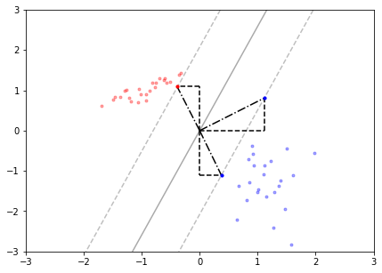
Support vector is just another way of referring to a point that lies nearest to the boundary. Note that geometric vectors are drawn from the origin of the vector space. The use of support vectors in drawing decision boundaries is effective because they maximize the decision margin (i.e. define a margin such that the nearest point in either class is as far away from the dividing hyperplane as possible). This helps the boundary generalize to new data, assuming the training data is representative.

支持向量只是引用最接近边界的点的另一种方式。注意，几何矢量是从矢量空间的原点绘制的。支持向量在绘制决策边界中的使用是有效的，因为它们最大化了决策余量(即定义一个余量，以使任一类中的最近点都尽可能远离分割超平面)。假设训练数据具有代表性，这有助于将边界推广到新数据。

This case of SVM classification would be referred to as “hard margin” because there are no points that fall inside the decision margin. In many cases of SVM classification, it makes more sense to use a “soft margin”, which would give “slack” to some points and allow them to encroach on the dividing region. This is useful because it is less sensitive to anomalies and class instances that overlap one another.

支持向量机分类的这种情况将被称为“硬边际”，因为没有点落在决策边际之内。在SVM分类的许多情况下，使用“软边距”会更有意义，这会给某些点“松弛”并允许它们侵占划分区域。这很有用，因为它对异常和彼此重叠的类实例不太敏感。

Now that we understand what support vectors are, let’s use them. The SVM algorithm is phrased as a constrained optimization problem; specifically one that uses inequality constraints. The problem takes the following form:

现在我们了解了什么是支持向量，让我们使用它们。 SVM算法被表述为约束优化问题。特别是使用不平等约束的该问题采用以下形式：

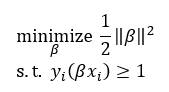
Here, β is a vector of coefficients and y ϵ {-1,1}. The dependent variable takes the form -1 or 1 instead of the usual 0 or 1 here so that we may formulate the “hinge” loss function used in solving the problem:

此处， β是系数和y ϵ {-1,1}的向量。因变量采用-1或1的形式，而不是通常的0或1的形式，以便我们可以公式化用于解决问题的“铰链”损失函数：

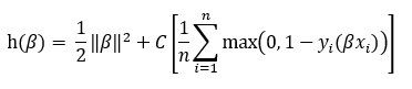
Here, the constraint has been moved into the objective function and is being regularized by the parameter C. Generally, a lower value of C will give a softer margin. Minimizing this loss function will yield a set of coefficients β =[β0, β1, … , βk] that look similar to a linear regression equation. Predictions are made according to the criteria:

此处，约束已移至目标函数，并通过参数C进行正则化。通常，较低的C值将提供较软的余量。最小化此损失函数将产生一组系数β= [β0，β1，…，βk] ，看起来与线性回归方程相似。根据以下条件进行预测：

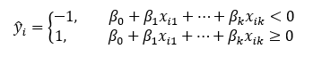
Put simply: if the predicted value is less than 0, the observation lies on one side of the decision boundary; if it is greater than or equal to 0, the observation lies on the other side of the boundary.

简而言之：如果预测值小于0，则观察值位于决策边界的一侧；如果它大于或等于0，则观察值位于边界的另一侧。

Now that we have defined the hinge loss function and the SVM optimization problem, let’s discuss one way of solving it.

现在我们已经定义了铰链损失函数和SVM优化问题，让我们讨论一种解决方法。

2.随机梯度下降 (2. Stochastic Gradient Descent)

There are several ways of solving optimization problems. One commonly used method in machine learning, mainly for its fast implementation, is called Gradient Descent. Gradient Descent is an iterative learning process where an objective function is minimized according to the direction of steepest ascent so that the best coefficients for modeling may be converged upon. While there are different versions of Gradient Descent that vary depending on how many training instances are used at each iteration, we will discuss Stochastic Gradient Descent (SGD).

有几种解决优化问题的方法。机器学习中一种主要用于快速实现的常用方法称为梯度下降。梯度下降是一种迭代学习过程，其中，根据最陡峭上升的方向将目标函数最小化，以便可以将用于建模的最佳系数收敛。虽然有不同版本的Gradient Descent(梯度下降)，具体取决于每次迭代使用多少个训练实例，但我们将讨论随机梯度下降(SGD)。

A gradient is a vector that contains every partial derivative of a function. Partial derivatives define how the slope of a function changes with respect to an infinitesimal change in one variable. A vector of all partial derivatives will define how the slope of a function changes with respect to changes in each of the variables. All of these derivatives taken together indicate which direction, with respect to the origin of the vector space, the function has the steepest slope in.

梯度是包含函数的每个偏导数的向量。偏导数定义函数的斜率相对于一个变量的无穷小变化如何变化。所有偏导数的向量将定义函数的斜率相对于每个变量的变化如何变化。所有这些导数加起来表示相对于向量空间的原点，函数的斜率最大。

SGD works by initializing a set of coefficients with random values, calculating the gradient of the loss function at a given point in the dataset, and updating those coefficients by taking a “step” of a defined size (given by the parameter η) in the opposite direction of the gradient. The algorithm iteratively updates the coefficients such that they are moving opposite the direction of steepest ascent (away from the maximum of the loss function) and toward the minimum, approximating a solution for the optimization problem. The algorithm follows this general form:

SGD的工作原理是初始化一组具有随机值的系数，计算数据集中给定点处的损失函数的梯度，并通过在参数集中采用定义大小(由参数η赋予)的“步长”来更新这些系数。渐变的相反方向。该算法迭代地更新系数，以使它们与最陡的上升方向(远离损失函数的最大值)相反并朝最小值的方向移动，从而逼近了优化问题的解决方案。该算法遵循以下一般形式：

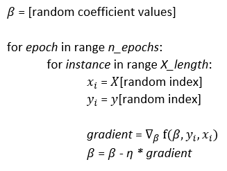
Here, η is the specified learning rate, n_epochs is the number of times the algorithm looks over the full dataset, f(β, yi, xi) is the loss function, and gradient is the collection of partial derivatives for every βi in the loss function evaluated at random instances of X and y.

在这里， η是指定的学习率， n_epochs是算法查看整个数据集的次数， f(β，yi，xi)是损失函数，并且梯度是损失中每个βi的偏导数的集合在X和y的随机实例处评估的函数。

SGD operates by using one randomly selected observation from the dataset at a time (different from regular Gradient Descent, which uses the entire dataset together). This is often preferred because it reduces the chances of the algorithm getting stuck in local minima instead of finding the global minimum. The stochastic nature of the points at which the function is evaluated allows the algorithm to “jump” out of any local minima that may exist. The figure below plots the trace of β as the algorithm iterates, eventually centering around the true value of the coefficients (denoted as a black point).

SGD通过一次从数据集中使用一个随机选择的观测值来进行操作(不同于常规的“梯度下降”，后者将整个数据集一起使用)。这通常是优选的，因为它减少了算法陷入局部最小值而不是找到全局最小值的机会。函数评估点的随机性质允许算法从可能存在的任何局部最小值中“跳出”。下图绘制了算法迭代时β的轨迹，最终以系数的真实值(表示为黑点)为中心。

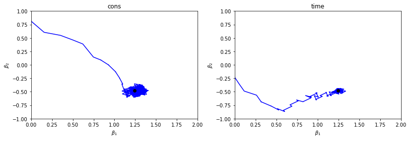
With a constant learning rate (the left-hand plot), each step the algorithm takes toward the minimum is of the same length. For this reason, the algorithm gets close to but never converges on the true value. With a time decaying learning rate (the right-hand plot), the steps get shorter as the algorithm continues to iterate. As the steps get smaller and smaller, the algorithm converges closer and closer to the true value. Centering and scaling data beforehand is another important step for convergence.

在学习率恒定的情况下(左侧图)，算法朝着最小值迈出的每一步都具有相同的长度。因此，该算法接近但从未收敛于真实值。在学习速率随时间递减的情况下(右侧图)，随着算法继续迭代，步骤变得更短。随着步长越来越小，算法收敛到越来越接近真实值。预先居中和缩放数据是收敛的另一个重要步骤。

With the SVM objective function in place and the process of SGD defined, we may now put the two together to perform classification.

有了SVM目标函数并定义了SGD的过程之后，我们现在可以将两者放在一起进行分类。

3.使用SGD优化SVM (3. Optimizing the SVM with SGD)

To use Stochastic Gradient Descent on Support Vector Machines, we must find the gradient of the hinge loss function. This will be easier if we rewrite the equation like this:

要在支持向量机上使用随机梯度下降，我们必须找到铰链损失函数的梯度。如果我们这样重写方程式，这将变得更加容易：

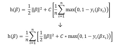
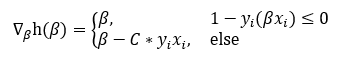
Taking the partial derivative of the bottom equation with respect to β yields the gradient:

取底方程相对于β的偏导数可得出梯度：

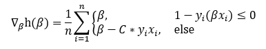
Now, because we are only calculating one instance at a time with Stochastic Gradient Descent, the gradient used in the algorithm is:

现在，由于我们每次仅使用随机梯度下降计算一次实例，因此算法中使用的梯度为：

Here, β =[β0, β1, … , βk]. With this gradient, the SGD algorithm described in section 2 must be modified slightly:

在此， β＝ [β0，β1，…，βk]。 使用此梯度，必须对第2节中描述的SGD算法进行一些修改：

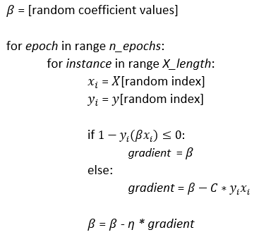
Here, C is the regularization parameter, η is the learning rate, and β is initialized as a vector of random values for coefficients. The figure below plots the results of this algorithm run on the data presented in section 1. The left-hand plot shows the trace of the two β coefficients as SGD iterates, and the right-hand plot shows the associated hinge loss of the model at each iteration.

在此， C是正则化参数， η是学习率， β初始化为系数的随机值向量。下图根据第1节中提供的数据绘制了该算法的结果。左图显示了SGD迭代时两个β系数的轨迹，右图显示了模型在以下位置的相关铰链损耗每次迭代。

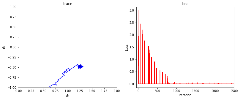
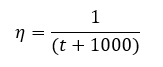
Note how on the first several iterations, the trace is far away from its convergent point and the loss is extremely high. As the algorithm continues, the trace converges and the loss falls to near 0. This SGD process has C set to 100, n_epochs set to 1000, and a learning schedule defined below, where t is the iteration number:

请注意，在前几次迭代中，走线是如何远离其收敛点的，而损耗却非常高。随着算法的继续，跟踪收敛，并且损失降到接近0。此SGD过程将C设置为100， n_epochs设置为1000，并且在下面定义了学习计划，其中t是迭代次数：

The estimated decision boundary is displayed below.

估计的决策边界显示在下面。

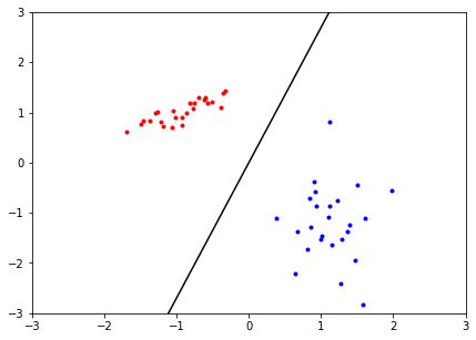
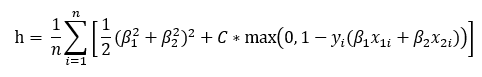
With this dataset, the SGD process appears to have done an excellent job of estimating the SVM decision boundary. We can confirm this solution by checking if the first and second order conditions of the optimization problem are satisfied. First, we define the objective function of the 2-variable hinge loss used:

使用此数据集，SGD过程似乎在估计SVM决策边界方面做得非常出色。我们可以通过检查是否满足优化问题的一阶和二阶条件来确认该解决方案。首先，我们定义所使用的2变量铰链损耗的目标函数：

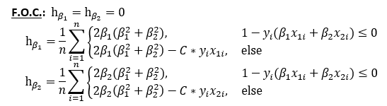
The first order conditions of this function are:

此函数的一阶条件为：

And the second order conditions are:

第二阶条件是：

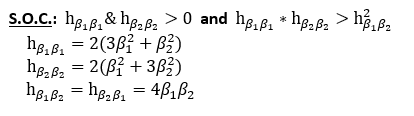
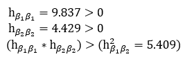
In evaluating the second order conditions at the coefficients determined by SGD (β1=1.252 and β2 =-0.464), we find that our coefficients do minimize the objective function:

在以SGD确定的系数( β1= 1.252和β2 = -0.464)评估二阶条件时，我们发现我们的系数确实使目标函数最小化：

Evaluating the first order conditions at our coefficients shows that we actually have not found a perfect solution to the optimization problem:

用系数评估一阶条件表明，实际上我们还没有找到优化问题的理想解决方案：

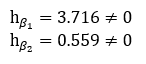
The failure of our coefficients to satisfy the first order conditions is due to the nature of SGD. The algorithm does not always converge on the true solution, especially if the parameters are not tuned perfectly. Almost always, SGD only approximates the true values of the solution.

我们的系数不能满足一阶条件是由于SGD的性质。该算法并不总是收敛于真实的解，尤其是在参数没有得到完美调整的情况下。 SGD几乎总是只近似解决方案的真实值。

Looking at the first order conditions and the plot of the decision boundary, we can conclude that the process used here still does a fairly good job — all things considered. In the context of machine learning, our solution has high accuracy and the decision boundary is robust. Despite an imperfect solution in the mathematical sense, SGD has derived a solid model.

查看一阶条件和决策边界图，我们可以得出结论，此处考虑的所有过程仍然可以很好地完成工作。在机器学习的背景下，我们的解决方案具有很高的准确性，并且决策边界很稳健。尽管在数学意义上解决方案不完善，但SGD仍推导出了实体模型。

结论 (Conclusion)

Many people have written very impressive blog posts about Support Vector Machines, Stochastic Gradient Descent, and different types of loss functions. As an individual studying data science myself, I find it extremely helpful that such a wealth of information is offered by those eager to share their knowledge. Whenever discouraged by one post that seems too complicated, there are always others to turn to that remedy my confusion.

许多人撰写了非常令人印象深刻的博客文章，内容涉及支持向量机，随机梯度下降以及不同类型的损失函数。作为一个自己学习数据科学的人，我发现非常有帮助的是那些渴望共享其知识的人可以提供如此丰富的信息。每当因一篇似乎过于复杂的文章而灰心时，总会有其他人转向该补救措施，以免引起我的困惑。

That being said, I recognize that I am far from the first on Towards Data Science to write about SVM problems and likely will not be the last. However, I’m throwing my hat in the ring in hopes that my perspective may be just what another aspiring data scientist is looking for.

话虽这么说，我认识到我距离撰写数据支持向量机问题的“迈向数据科学”还很远，而且可能不会是最后一个。但是，我满怀希望，希望我的观点可能正是另一位有抱负的数据科学家正在寻找的观点。

While this post does not touch on very advanced topics in SVM, exploration of such topics can be found in countless other blog posts, textbooks, and scholarly articles. I hope that my contribution to the expanse of resources on Support Vector Machines has been helpful. If not, I have linked more resources that I have found to be useful below.

尽管本文不涉及SVM中非常高级的主题，但可以在无数其他博客文章，教科书和学术文章中找到对此类主题的探索。我希望我对支持向量机资源的扩展能有所帮助。如果没有，我已经链接了更多我认为在下面有用的资源。