Kaggle竞赛 Flower Classification on TPU 使用TPU对104种花朵进行分类 中文注释【深度学习TPU+TensorFlow2+Keras+ResNet】

目录

开发环境

0 前言

1 导入所需库

2 检测TPU环境

3 配置TPU、访问路径等

4 辅助函数

4.1 可视化函数

4.2 数据集函数

4.3 模型函数

4.4 数据及可视化

 5 训练模型

5.1 创建模型并加载到TPU

5.2 绘制损失函数

5.3 绘制混淆矩阵

5.4 预测

5.5 验证

6 结果展示

开发环境

作者：粥粥坠腻害

时间：2023年9月28日

集成开发环境：Kaggle平台

0 前言

本竞赛英文全称
Flower Classification with TPUs
Use TPUs to classify 104 types of flowers

以下为比赛的描述：
在这场比赛中，您面临的挑战是建立一个机器学习模型，该模型可识别图像。
数据集中的花朵类型（为简单起见，我们坚持使用100多种类型的花朵）。

数据集：
12753个训练图像，3712个验证图像，7382个未标记的测试图像
选用的数据为：
在这次比赛中，我们根据来自五个不同公共数据集的花卉图像对104种花卉进行分类。有些种类非常狭窄，只包含一个特定的花的子种类（例如粉红报春花），而其他种类包含许多子种类（例如野生玫瑰）。
这种竞赛的不同之处在于以TFRecord格式提供图像。 TFRecord格式是Tensorflow中经常使用的容器格式，用于对数据数据文件进行分组和分片以获得最佳训练性能。每个文件都包含许多图像的id，标签（样本数据，用于训练数据）和img（数组形式的实际像素）信息。

• train/*.tfrec - 训练集，包括标签。
• val/*.tfrec - 验证集。预分割训练样本，带有帮助检查您的模型在TPU上的性能的标签。这种分割是按标签分层的。
• test/*.tfrec - 测试集，不带标签的样本 - 您将预测这些花属于哪一类。
• sample_submission.csv - 格式正确的示例提交文件
  • id-每个样本的唯一id。
  • 标记（在训练数据中）样本所代表的花的类别。

比赛最终分数由70%给定的测试集（我们能拿到的test数据）和30%其他测试集决定，我们模型可能在这70%上表现好，在另外30%就差了，故你最终的提交分数可能会低于你自己测试分数。

1 导入所需库

# 导入需要的包
import math, re, os
import tensorflow as tf
import numpy as np
from matplotlib import pyplot as plt
from kaggle_datasets import KaggleDatasets # Kaggle数据集
from tensorflow.keras.applications import EfficientNetB7   # 导入efficientnet模型
# 从python的sklearn机器学习中导入f1值、精度、召回率和混淆矩阵
from sklearn.metrics import f1_score, precision_score, recall_score, confusion_matrix  print("Tensorflow version " + tf.__version__) # 检查tensorflow的版本

2 检测TPU环境

try:# TPU检测。 如果设置了TPU_NAME环境变量，则不需要任何参数。 在Kaggle上，情况总是如此。tpu = tf.distribute.cluster_resolver.TPUClusterResolver()  # 获取默认的 TensorFlow 分布式策略print('Running on TPU ', tpu.master())
except ValueError:tpu = Noneif tpu:tf.config.experimental_connect_to_cluster(tpu)  # 连接到TPU集群tf.tpu.experimental.initialize_tpu_system(tpu)  # 连接到TPU系统strategy = tf.distribute.TPUStrategy(tpu)  # 创建TPU分布式策略
else:strategy = tf.distribute.get_strategy() # Tensorflow 中的默认分配策略。 适用于 CPU 和单 GPU。print("REPLICAS: ", strategy.num_replicas_in_sync) # 输出副本数

Running on TPU  
INFO:tensorflow:Deallocate tpu buffers before initializing tpu system.
INFO:tensorflow:Initializing the TPU system: local
INFO:tensorflow:Finished initializing TPU system.
INFO:tensorflow:Found TPU system:
INFO:tensorflow:*** Num TPU Cores: 8
INFO:tensorflow:*** Num TPU Workers: 1
INFO:tensorflow:*** Num TPU Cores Per Worker: 8
INFO:tensorflow:*** Available Device: _DeviceAttributes(/job:localhost/replica:0/task:0/device:CPU:0, CPU, 0, 0)
INFO:tensorflow:*** Available Device: _DeviceAttributes(/job:localhost/replica:0/task:0/device:TPU:0, TPU, 0, 0)
INFO:tensorflow:*** Available Device: _DeviceAttributes(/job:localhost/replica:0/task:0/device:TPU:1, TPU, 0, 0)
INFO:tensorflow:*** Available Device: _DeviceAttributes(/job:localhost/replica:0/task:0/device:TPU:2, TPU, 0, 0)
INFO:tensorflow:*** Available Device: _DeviceAttributes(/job:localhost/replica:0/task:0/device:TPU:3, TPU, 0, 0)
INFO:tensorflow:*** Available Device: _DeviceAttributes(/job:localhost/replica:0/task:0/device:TPU:4, TPU, 0, 0)
INFO:tensorflow:*** Available Device: _DeviceAttributes(/job:localhost/replica:0/task:0/device:TPU:5, TPU, 0, 0)
INFO:tensorflow:*** Available Device: _DeviceAttributes(/job:localhost/replica:0/task:0/device:TPU:6, TPU, 0, 0)
INFO:tensorflow:*** Available Device: _DeviceAttributes(/job:localhost/replica:0/task:0/device:TPU:7, TPU, 0, 0)
INFO:tensorflow:*** Available Device: _DeviceAttributes(/job:localhost/replica:0/task:0/device:TPU_SYSTEM:0, TPU_SYSTEM, 0, 0)
REPLICAS:  8

3 配置TPU、访问路径等

AUTO = tf.data.experimental.AUTOTUNE # 让程序自动选择最优的线程并行个数# 从TPU创建部署
tpu = tf.distribute.cluster_resolver.TPUClusterResolver() # 如果先前设置好了ＴＰＵ＿ＮＡＭＥ环境变量，不需要再给参数．
tf.config.experimental_connect_to_cluster(tpu) # 配置实验连接到群集
tf.tpu.experimental.initialize_tpu_system(tpu) # 初始化tpu系统
strategy = tf.distribute.TPUStrategy(tpu) # 设置TPU部署# 比赛数据访问
# TPU直接从Google Cloud Storage（GCS）读取数据。
# 该Kaggle实用程序会将数据集复制到与TPU并置的GCS存储桶中。
# 如果笔记本有多个数据集，
# 您可以将特定数据集的名称传递给get_gcs_path函数。
# 数据集的名称是其安装目录的名称。
# 使用！ls / kaggle / input /列出附加的数据集。GCS_DS_PATH = KaggleDatasets().get_gcs_path() #设置Kaggle数据的访问路径# ConfigurationIMAGE_SIZE = [512, 512] # 输入图像尺寸
EPOCHS = 20 # 配置模型训练的轮次
BATCH_SIZE = 16 * strategy.num_replicas_in_sync # 设置每个小批量的大小

INFO:tensorflow:Deallocate tpu buffers before initializing tpu system.
WARNING:tensorflow:TPU system local has already been initialized. Reinitializing the TPU can cause previously created variables on TPU to be lost.
INFO:tensorflow:Initializing the TPU system: local
INFO:tensorflow:Finished initializing TPU system.
INFO:tensorflow:Found TPU system:
INFO:tensorflow:*** Num TPU Cores: 8
INFO:tensorflow:*** Num TPU Workers: 1
INFO:tensorflow:*** Num TPU Cores Per Worker: 8
INFO:tensorflow:*** Available Device: _DeviceAttributes(/job:localhost/replica:0/task:0/device:CPU:0, CPU, 0, 0)
INFO:tensorflow:*** Available Device: _DeviceAttributes(/job:localhost/replica:0/task:0/device:TPU:0, TPU, 0, 0)
INFO:tensorflow:*** Available Device: _DeviceAttributes(/job:localhost/replica:0/task:0/device:TPU:1, TPU, 0, 0)
INFO:tensorflow:*** Available Device: _DeviceAttributes(/job:localhost/replica:0/task:0/device:TPU:2, TPU, 0, 0)
INFO:tensorflow:*** Available Device: _DeviceAttributes(/job:localhost/replica:0/task:0/device:TPU:3, TPU, 0, 0)
INFO:tensorflow:*** Available Device: _DeviceAttributes(/job:localhost/replica:0/task:0/device:TPU:4, TPU, 0, 0)
INFO:tensorflow:*** Available Device: _DeviceAttributes(/job:localhost/replica:0/task:0/device:TPU:5, TPU, 0, 0)
INFO:tensorflow:*** Available Device: _DeviceAttributes(/job:localhost/replica:0/task:0/device:TPU:6, TPU, 0, 0)
INFO:tensorflow:*** Available Device: _DeviceAttributes(/job:localhost/replica:0/task:0/device:TPU:7, TPU, 0, 0)
INFO:tensorflow:*** Available Device: _DeviceAttributes(/job:localhost/replica:0/task:0/device:TPU_SYSTEM:0, TPU_SYSTEM, 0, 0)
get_gcs_path is not required on TPU VMs which can directly use Kaggle datasets, using path: /kaggle/input/tpu-getting-started

# 配置不同大小图片的路径
GCS_PATH_SELECT = { # available image sizes192: GCS_DS_PATH + '/tfrecords-jpeg-192x192',224: GCS_DS_PATH + '/tfrecords-jpeg-224x224',331: GCS_DS_PATH + '/tfrecords-jpeg-331x331',512: GCS_DS_PATH + '/tfrecords-jpeg-512x512'
}
GCS_PATH = GCS_PATH_SELECT[IMAGE_SIZE[0]]TRAINING_FILENAMES = tf.io.gfile.glob(GCS_PATH + '/train/*.tfrec') # 训练集路径
VALIDATION_FILENAMES = tf.io.gfile.glob(GCS_PATH + '/val/*.tfrec') # 验证集路径
TEST_FILENAMES = tf.io.gfile.glob(GCS_PATH + '/test/*.tfrec') # 测试集路径 predictions on this dataset should be submitted for the competition

Kaggle为这个竞赛提供了4种不同尺寸的数据集，本文选择的是512x512尺寸。

# 104种花的名称
CLASSES = ['pink primrose',    'hard-leaved pocket orchid', 'canterbury bells', 'sweet pea',     'wild geranium',     'tiger lily',           'moon orchid',              'bird of paradise', 'monkshood',        'globe thistle',         # 00 - 09'snapdragon',       "colt's foot",               'king protea',      'spear thistle', 'yellow iris',       'globe-flower',         'purple coneflower',        'peruvian lily',    'balloon flower',   'giant white arum lily', # 10 - 19'fire lily',        'pincushion flower',         'fritillary',       'red ginger',    'grape hyacinth',    'corn poppy',           'prince of wales feathers', 'stemless gentian', 'artichoke',        'sweet william',         # 20 - 29'carnation',        'garden phlox',              'love in the mist', 'cosmos',        'alpine sea holly',  'ruby-lipped cattleya', 'cape flower',              'great masterwort', 'siam tulip',       'lenten rose',           # 30 - 39'barberton daisy',  'daffodil',                  'sword lily',       'poinsettia',    'bolero deep blue',  'wallflower',           'marigold',                 'buttercup',        'daisy',            'common dandelion',      # 40 - 49'petunia',          'wild pansy',                'primula',          'sunflower',     'lilac hibiscus',    'bishop of llandaff',   'gaura',                    'geranium',         'orange dahlia',    'pink-yellow dahlia',    # 50 - 59'cautleya spicata', 'japanese anemone',          'black-eyed susan', 'silverbush',    'californian poppy', 'osteospermum',         'spring crocus',            'iris',             'windflower',       'tree poppy',            # 60 - 69'gazania',          'azalea',                    'water lily',       'rose',          'thorn apple',       'morning glory',        'passion flower',           'lotus',            'toad lily',        'anthurium',             # 70 - 79'frangipani',       'clematis',                  'hibiscus',         'columbine',     'desert-rose',       'tree mallow',          'magnolia',                 'cyclamen ',        'watercress',       'canna lily',            # 80 - 89'hippeastrum ',     'bee balm',                  'pink quill',       'foxglove',      'bougainvillea',     'camellia',             'mallow',                   'mexican petunia',  'bromelia',         'blanket flower',        # 90 - 99'trumpet creeper',  'blackberry lily',           'common tulip',     'wild rose']

4 辅助函数

4.1 可视化函数

# 展示训练和验证曲线，也就是损失和准确率随轮次的变化
def display_training_curves(training, validation, title, subplot):if subplot % 10 == 1: # 在第一次调用该函数时设置子图plt.subplots(figsize=(10,10), facecolor='#F0F0F0')plt.tight_layout()  # 使子图排列紧密ax = plt.subplot(subplot) # 设置子图ax.set_facecolor('#F8F8F8') # 设置背景颜色ax.plot(training) # 画训练集的曲线ax.plot(validation) # 画测试集的曲线ax.set_title('model '+ title)ax.set_ylabel(title) # 设置y轴标题
#     ax.set_ylim(0.28,1.05) # 设置y轴刻度范围ax.set_xlabel('epoch') # 设置x轴标题ax.legend(['train', 'valid.']) # 设置图例# 绘制混淆矩阵
def display_confusion_matrix(cmat, score, precision, recall):plt.figure(figsize=(15,15))  # 设置画布大小ax = plt.gca() # 返回当前axes(matplotlib.axes.Axes) 获取当前子图ax.matshow(cmat, cmap='Reds') # 绘制矩阵ax.set_xticks(range(len(CLASSES)))  # 根据花朵类别数（其实就是104）设置x轴范围ax.set_xticklabels(CLASSES, fontdict={'fontsize': 7}) # 设置x轴下标字体的大小plt.setp(ax.get_xticklabels(), rotation=45, ha="left", rotation_mode="anchor") # 更换x轴下标角度ax.set_yticks(range(len(CLASSES)))  # 根据花朵类别数（其实就是104）设置y轴范围ax.set_yticklabels(CLASSES, fontdict={'fontsize': 7}) # 设置y轴下标字体的大小plt.setp(ax.get_yticklabels(), rotation=45, ha="right", rotation_mode="anchor") # 更换y轴下标角度titlestring = ""if score is not None:titlestring += 'f1 = {:.3f} '.format(score) # 更改格式为有3位小数的浮点数if precision is not None:titlestring += '\nprecision = {:.3f} '.format(precision) # 更改格式为有3位小数的浮点数if recall is not None:titlestring += '\nrecall = {:.3f} '.format(recall) # 更改格式为有3位小数的浮点数if len(titlestring) > 0:ax.text(101, 1, titlestring, fontdict={'fontsize': 18, 'horizontalalignment':'right', 'verticalalignment':'top', 'color':'#804040'}) #添加文本注释plt.show()

# 设置numpy数组基本属性，设置显示15个数字，用于插入换行符的每行字符数（默认为75）。
# 当数组数目过大时，设置显示几个数字，其余用省略号
# 用于插入换行符的每行字符数（默认为75）。
np.set_printoptions(threshold=15, linewidth=80)# 将小批量图片和标签处理为numpy向量格式
def batch_to_numpy_images_and_labels(data):images, labels = data numpy_images = images.numpy() # 将图像转换为numpy向量格式numpy_labels = labels.numpy() # 将label标签转换为numpy向量格式if numpy_labels.dtype == object: # 在这种情况下为二进制字符串，它们是图像ID字符串numpy_labels = [None for _ in enumerate(numpy_images)]# 如果没有标签，只有图像ID，则对标签返回None（测试数据就是这种情况）return numpy_images, numpy_labels# 把实际类型和模型预测出来的模型一起显示在图片上方，这是用给验证集的，当对验证集预测完标签后和验证集的实际标签进行比较
# label,图片中花朵的实际类别
# current_label，当前我们预测的类别
def title_from_label_and_target(label, current_label):# 如果没有预测的类别，则返回实际类别，比如训练集if current_label is None:return CLASSES[label], Truecurrent = (label == current_label) # 判断一下实际类别和我们预测的类别是否一致# 如果一致，则返回OK，不一致则返回NO加实际类别return "{} [{}{}{}]".format(CLASSES[label], 'OK' if current else 'NO', u"\u2192" if not current else '',CLASSES[current_label] if not current else ''), current# 绘制一朵花
def display_one_flower(image, title, subplot, red=False, titlesize=16):plt.subplot(*subplot)plt.axis('off') # 不显示坐标尺寸plt.imshow(image) # 函数负责对图像进行处理，并显示其格式；而plt.show()则是将plt.imshow()处理后的函数显示出来。if len(title) > 0:#绘制图片的标题plt.title(title, fontsize=int(titlesize) if not red else int(titlesize/1.2), color='red' if red else 'black', fontdict={'verticalalignment':'center'}, pad=int(titlesize/1.5))return (subplot[0], subplot[1], subplot[2]+1)# 展示小批量图片，我们在下面的代码中经常展示20张照片
def display_batch_of_images(databatch, predictions=None):"""This will work with:display_batch_of_images(images)    只展示图片 测试集需要这个display_batch_of_images(images, predictions) 展示图片加预测的类别 测试集需要这个display_batch_of_images((images, labels)) 展示图片加实际标签 训练集需要这个display_batch_of_images((images, labels), predictions) #展示图片+实际类别+预测类别 验证集需要这个，因为验证集既有实际标签，也会进行预测"""# 读取图片和实际标签数据，而且这些数据被转换成numpy向量的格式images, labels = batch_to_numpy_images_and_labels(databatch)# 如果没有实际标签，比如测试集，那么我们需要将labels变量设为每个元素都为noneif labels is None:labels = [None for _ in enumerate(images)]# 删除不适合矩形的数据，即一次只显示正好满足矩形数量的图片rows = int(math.sqrt(len(images)))cols = len(images) // rows# 画布大小和间距FIGSIZE = 13.0SPACING = 0.1subplot=(rows,cols,1)if rows < cols:# 如果行大于列plt.figure(figsize=(FIGSIZE, FIGSIZE / cols * rows))else:plt.figure(figsize=(FIGSIZE / rows * cols, FIGSIZE))# 显示for i, (image, label) in enumerate(zip(images[:rows * cols], labels[:rows * cols])):title = '' if label is None else CLASSES[label]correct = Trueif predictions is not None:title, correct = title_from_label_and_target(predictions[i], label)dynamic_titlesize = FIGSIZE * SPACING / max(rows,cols) * 40 + 3 # 经过测试可以在1x1到10x10图像上工作的魔术公式subplot = display_one_flower(image, title, subplot, not correct, titlesize=dynamic_titlesize)# 布局plt.tight_layout()if label is None and predictions is None:plt.subplots_adjust(wspace=0, hspace=0)else:plt.subplots_adjust(wspace=SPACING, hspace=SPACING)plt.show()

4.2 数据集函数

# 准备图像数据
def decode_image(image_data):image = tf.image.decode_jpeg(image_data, channels=3) # 将图片解码# 之前训练图像保存在一个 uint8 类型的数组中，取值区间为 [0, 255]。我们需要将其变换为一个 float32 数组，其新取值范围为 0~1。# 将图片转换为[0，1]范围内的浮点数image = tf.cast(image, tf.float32) / 255.0  image = tf.reshape(image, [*IMAGE_SIZE, 3]) # TPU所需的精确的大小return image# 读取带有标签的TFRecord 格式文件
def read_labeled_tfrecord(example):LABELED_TFREC_FORMAT = {"image": tf.io.FixedLenFeature([], tf.string), # tf.string means bytestring"class": tf.io.FixedLenFeature([], tf.int64),  # shape [] means single element}example = tf.io.parse_single_example(example, LABELED_TFREC_FORMAT)image = decode_image(example['image'])label = tf.cast(example['class'], tf.int32)return image, label # returns a dataset of (image, label) pairs# 读取没有标签的TFRecord 格式文件
def read_unlabeled_tfrecord(example):UNLABELED_TFREC_FORMAT = {"image": tf.io.FixedLenFeature([], tf.string), # tf.string means bytestring"id": tf.io.FixedLenFeature([], tf.string),  # shape [] means single element# class is missing, this competitions's challenge is to predict flower classes for the test dataset}example = tf.io.parse_single_example(example, UNLABELED_TFREC_FORMAT)image = decode_image(example['image'])idnum = example['id']return image, idnum # returns a dataset of image(s)# 加载数据集
# 这三个参数分别为：文件路径、是否有标签、是否按顺序（就是要不要把数据顺序打乱）
def load_dataset(filenames, labeled=True, ordered=False):# 从TFRecords读取。 为了获得最佳性能，请一次从多个文件中读取数据，而不考虑数据顺序。 顺序无关紧要，因为无论如何我们都会对数据进行混洗。ignore_order = tf.data.Options()if not ordered:ignore_order.experimental_deterministic = False # 禁用顺序，提高速度dataset = tf.data.TFRecordDataset(filenames, num_parallel_reads=AUTO)  # 自动交错读取多个文件dataset = dataset.with_options(ignore_order) # 在流入数据后立即使用数据，而不是按原始顺序使用dataset = dataset.map(read_labeled_tfrecord if labeled else read_unlabeled_tfrecord, num_parallel_calls=AUTO)# 如果标记为True则返回（图像，label）对的数据集，如果标记为False，则返回（图像，id）对的数据集return dataset# 按水平 (从左向右) 随机翻转图像.返回图片的参数image和label
def data_augment(image, label, seed=2020):# TensorFlow函数：tf.image.random_flip_left_right# 按水平 (从左向右) 随机翻转图像.# 以1比2的概率,输出image沿着第二维翻转的内容,即,width.否则按原样输出图像.# 参数：# image：形状为[height, width, channels]的三维张量.# seed：一个Python整数,用于创建一个随机种子.查看tf.set_random_seed行为.# 返回：一个与image具有相同类型和形状的三维张量.image = tf.image.random_flip_left_right(image, seed=seed)#     image = tf.image.random_flip_up_down(image, seed=seed)
#     image = tf.image.random_brightness(image, 0.1, seed=seed)
#     image = tf.image.random_jpeg_quality(image, 85, 100, seed=seed)
#     image = tf.image.random_saturation(image, 0, 2)return image, label   # 获取训练集
def get_training_dataset():# 加载训练集，第一个参数为训练集路径，第二个参数表示有标签dataset = load_dataset(TRAINING_FILENAMES, labeled=True)# 将数据转换并行化# num_parallel_calls 参数选择最佳值取决于您的硬件、训练数据的特征（例如其大小和形状）、Map 功能的成本以及在 CPU 上同时进行的其他处理；dataset = dataset.map(data_augment, num_parallel_calls=AUTO)# 重复此数据集count次数# 函数形式：repeat(count=None)# 参数count:(可选）表示数据集应重复的次数。默认行为（如果count是None或-1）是无限期重复的数据集。dataset = dataset.repeat() # 数据集必须重复几个轮次dataset = dataset.shuffle(2048) # 将数据打乱，括号中数值越大，混乱程度越大dataset = dataset.batch(BATCH_SIZE) # 按照顺序将小批量中样本数目行数据合成一个小批量，最后一个小批量可能小于20# pipeline（管道）读取数据，在训练时预取下一批（自动调整预取缓冲区大小）dataset = dataset.prefetch(AUTO) return dataset# 获取验证集
def get_validation_dataset(ordered=False):# 加载验证集，第一个参数为验证集路径，第二个参数表示有标签，第三个参数为不按照顺序dataset = load_dataset(VALIDATION_FILENAMES, labeled=True, ordered=ordered)dataset = dataset.batch(BATCH_SIZE) ## 按照顺序将小批量中样本数目行数据合成一个小批量，最后一个小批量可能小于20dataset = dataset.cache() # 使用.cache()方法：当计算缓存空间足够时，将preprocess的数据存储在缓存空间中将大幅提高计算速度。# pipeline（管道）读取数据，在训练时预取下一批（自动调整预取缓冲区大小）dataset = dataset.prefetch(AUTO)  return dataset# 将训练集和验证集合并
def get_train_valid_datasets():dataset = load_dataset(TRAINING_FILENAMES + VALIDATION_FILENAMES, labeled=True)# 将数据转换并行化# 加载训练集，第一个参数为训练集路径，第二个参数表示有标签dataset = dataset.map(data_augment, num_parallel_calls=AUTO)# 重复此数据集count次数# 函数形式：repeat(count=None)# 参数count:(可选）表示数据集应重复的次数。默认行为（如果count是None或-1）是无限期重复的数据集。dataset = dataset.repeat() # 数据集必须重复几个轮次dataset = dataset.shuffle(2048) # 将数据打乱，括号中数值越大，混乱程度越大dataset = dataset.batch(BATCH_SIZE)# pipeline（管道）读取数据，在训练时预取下一批（自动调整预取缓冲区大小）dataset = dataset.prefetch(AUTO)return dataset# 获取测试集
def get_test_dataset(ordered=False):dataset = load_dataset(TEST_FILENAMES, labeled=False, ordered=ordered)dataset = dataset.batch(BATCH_SIZE)# pipeline（管道）读取数据，在训练时预取下一批（自动调整预取缓冲区大小）dataset = dataset.prefetch(AUTO)return dataset# 计算数据集样本数目
def count_data_items(filenames):# 数据集的数量以.tfrec文件的名称编写，即flowers00-230.tfrec = 230个数据项n = [int(re.compile(r"-([0-9]*)\.").search(filename).group(1)) for filename in filenames]return np.sum(n)

对数据集使用数据增强可以使得模型更具鲁棒性，即提升模型的性能。但Kaggle提供的免费TPU的内存不足以正常加载数据增强后的数据集，故本文只保留了能正常加载的数据增强后的数据集定义，若读者能申请到更大内存的TPU额度，可去除注释。

4.3 模型函数

# LearningRate Function 自己编写的学习率函数
def lrfn(epoch):LR_START = 0.00001 # 初始学习率LR_MAX = 0.00005 * strategy.num_replicas_in_sync # 最大学习率LR_MIN = 0.00001 # 最小学习率LR_RAMPUP_EPOCHS = 5  # 学习率从初始值线性增加到最大值的轮次数LR_SUSTAIN_EPOCHS = 0  # 学习率保持在最大值的轮次数LR_EXP_DECAY = .8  # 学习率从最大值指数衰减到最小值的衰减率if epoch < LR_RAMPUP_EPOCHS:lr = (LR_MAX - LR_START) / LR_RAMPUP_EPOCHS * epoch + LR_STARTelif epoch < LR_RAMPUP_EPOCHS + LR_SUSTAIN_EPOCHS:lr = LR_MAXelse:lr = (LR_MAX - LR_MIN) * LR_EXP_DECAY ** (epoch - LR_RAMPUP_EPOCHS - LR_SUSTAIN_EPOCHS) + LR_MINreturn lr

4.4 数据及可视化

# 数据展示
print("Training data shapes:")
# 输出训练集前3个小批量的图像数据形状、标签形状
for image, label in get_training_dataset().take(3):print(image.numpy().shape, label.numpy().shape)
# 训练数据标签示例
print("Training data label examples:", label.numpy())print("Validation data shapes:")
# 输出验证集前3个小批量的图像数据形状、标签形状
for image, label in get_validation_dataset().take(3):print(image.numpy().shape, label.numpy().shape)
# 验证数据标签示例
print("Validation data label examples:", label.numpy())print("Test data shapes:")
# 输出测试集前3个小批量的图像数据形状、标签形状
for image, idnum in get_test_dataset().take(3):print(image.numpy().shape, idnum.numpy().shape)
# 测试集的id示例
print("Test data IDs:", idnum.numpy().astype('U')) # U=unicode string

Training data shapes:
(128, 512, 512, 3) (128,)
(128, 512, 512, 3) (128,)
(128, 512, 512, 3) (128,)
Training data label examples: [79 45 80 ... 74 62 32]
Validation data shapes:
(128, 512, 512, 3) (128,)
(128, 512, 512, 3) (128,)
(128, 512, 512, 3) (128,)
Validation data label examples: [103  47  53 ...  45  87  73]
Test data shapes:
(128, 512, 512, 3) (128,)
(128, 512, 512, 3) (128,)
(128, 512, 512, 3) (128,)
Test data IDs: ['3da7e8585' '705344bd8' '03c9840a9' ... '44e4c1b98' '6939eb499' 'eb64f3c3f']

# 查看训练集
training_dataset = get_training_dataset() # 获取训练集
training_dataset = training_dataset.unbatch().batch(20) # 将训练集分成大小为20的小批量
train_batch = iter(training_dataset) # 首先获得Iterator对象

# 再次运行该单元格以获取下一组图像
display_batch_of_images(next(train_batch))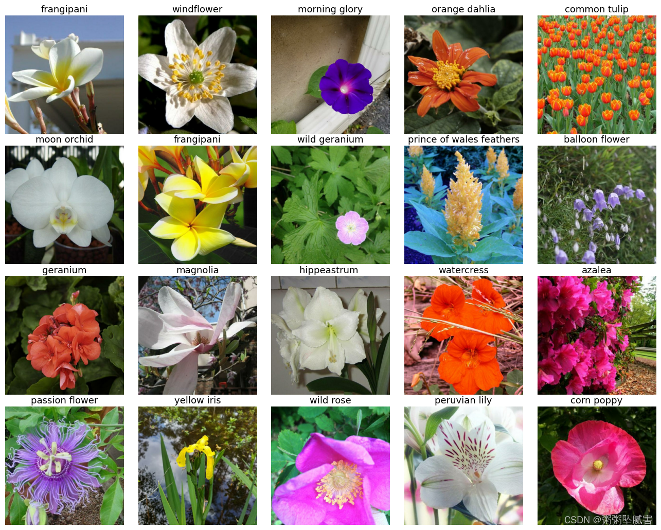

# 查看测试集
test_dataset = get_test_dataset() #通过一个函数来获取测试集
test_dataset = test_dataset.unbatch().batch(20) # 将训练集分成大小为20的小批量
test_batch = iter(test_dataset) # 首先获得Iterator对象

# 再次运行该单元格以获取下一组图像
display_batch_of_images(next(test_batch))

 5 训练模型

NUM_TRAINING_IMAGES = count_data_items(TRAINING_FILENAMES) # 训练集样本数目
NUM_VALIDATION_IMAGES = count_data_items(VALIDATION_FILENAMES) # 验证集样本数目
NUM_TEST_IMAGES = count_data_items(TEST_FILENAMES) # 测试集样本数目
STEPS_PER_EPOCH = NUM_TRAINING_IMAGES // BATCH_SIZE # 每轮次中的步数=训练集样本数除以每个小批量中样本数目
# 输出训练集、验证集和测试集的数目
print('Dataset: {} training images, {} validation images, {} unlabeled test images'.format(NUM_TRAINING_IMAGES, NUM_VALIDATION_IMAGES, NUM_TEST_IMAGES))

Dataset: 12753 training images, 3712 validation images, 7382 unlabeled test images

5.1 创建模型并加载到TPU

本文选择了EfficientNetB4、EfficientNetB7、ResNet50和ResNet101模型作为对比。虽然这四种模型在这个数据集上的表现均十分优异（准确率均达到了100%），但提交后的发现ResNet系列模型的性能最佳（准确率逼近95%），而EfficientNetB4的性能最差（准确率只有80%+）。（使用不同的模型仅在模型定义处的代码不同，这里只给出ResNet101模型定义的代码，其他模型定义代码读者可仿照自行更换）

from tensorflow.keras.layers import GlobalAveragePooling2D, Dense
from tensorflow.keras.models import Sequential
from tensorflow.keras.optimizers import Adam
from tensorflow.keras.losses import SparseCategoricalCrossentropy
from tensorflow.keras.metrics import SparseCategoricalAccuracy# 创建模型并加载到TPU
with strategy.scope():# 创建ResNet-101模型，并加载预训练权重resnet101 = tf.keras.applications.ResNet101(weights='imagenet', include_top=False, input_shape=(512, 512, 3))# 创建模型model = tf.keras.Sequential([ #Sequential类（仅用于层的线性堆叠，这是目前最常见的网络架构）resnet101, # ResNet101模型tf.keras.layers.GlobalAveragePooling2D(), #全局平均池# len(CLASSES)：表示这个层将返回一个大小为类别个数（104）的张量# activation='softmax'：表示这个层将返回图片在104个类别上的概率，其中最大的概率表示这个图片的预测类别# softmax激活函数的本质就是将一个K维的任意实数向量压缩（映射）成另一个K维的实数向量，其中向量中的每个元素取值都介于（0，1）之间并且和为1。# 在多分类单标签问题中，可以用softmax作为最后的激活层，取概率最高的作为结果tf.keras.layers.Dense(len(CLASSES), activation='softmax')])# 编译模型model.compile(optimizer=tf.keras.optimizers.Adam(), #优化器：Adam 是一种可以替代传统随机梯度下降（SGD）过程的一阶优化算法，它能基于训练数据迭代地更新神经网络权重# 损失函数：# 对于多分类问题，可以用分类交叉熵（categorical crossentropy）或稀疏分类交叉熵（sparse_categorical_crossentropy）损失函数# 这个sparse_categorical_crossentropy损失函数在数学上与 categorical_crossentropy 完全相同，# 如果目标是 one-hot 编码的，那么使用 categorical_crossentropy 作为损失；# 如果目标是整数，那么使用 sparse_categorical_crossentropy 作为损失。loss = SparseCategoricalCrossentropy(),, metrics=[SparseCategoricalAccuracy()] # 监控指标：分类准确率)# 输出模型摘要model.summary()

Model: "sequential"
_________________________________________________________________Layer (type)                Output Shape              Param #   
=================================================================resnet101 (Functional)      (None, 16, 16, 2048)      42658176  global_average_pooling2d_1   (None, 2048)             0         (GlobalAveragePooling2D)                                        dense_1 (Dense)             (None, 104)               213096    =================================================================
Total params: 42,871,272
Trainable params: 42,765,928
Non-trainable params: 105,344
_________________________________________________________________

# scheduler = tf.keras.callbacks.ReduceLROnPlateau(patience=3, verbose=1)
# 作为回调函数的一员,LearningRateScheduler 可以按照epoch的次数自动调整学习率,
# 参数：
# schedule：一个函数，它将一个epoch索引作为输入（整数，从0开始索引）并返回一个新的学习速率作为输出（浮点数）。
# 我们这里用lrfn（epoch）函数
# verbose：int；当其为0时，保持安静；当其为1时，表示更新消息。
lr_schedule = tf.keras.callbacks.LearningRateScheduler(lrfn, verbose=1) # 训练模型
history = model.fit(get_train_valid_datasets(),  # 获取训练集steps_per_epoch=STEPS_PER_EPOCH, # 设置每轮的步数epochs=EPOCHS,  # 设置轮次callbacks=[lr_schedule], # 设置回调函数validation_data=get_validation_dataset() # 设置验证集
)

5.2 绘制损失函数

# 画出训练集和验证集随轮次变化的损失和准确率
display_training_curves(history.history['loss'], history.history['val_loss'], 'loss', 211) #损失曲线
display_training_curves(history.history['sparse_categorical_accuracy'], history.history['val_sparse_categorical_accuracy'], 'accuracy', 212) #准确率曲线

5.3 绘制混淆矩阵

# 因为我们要分割数据集并分别对图像和标签进行迭代，所以顺序很重要。
cmdataset = get_validation_dataset(ordered=True)  # 验证集
images_ds = cmdataset.map(lambda image, label: image)  # 图像集
labels_ds = cmdataset.map(lambda image, label: label).unbatch() # 标签集 
cm_correct_labels = next(iter(labels_ds.batch(NUM_VALIDATION_IMAGES))).numpy() # get everything as one batch
cm_probabilities = model.predict(images_ds) # 图片在104个类别上的概率
cm_predictions = np.argmax(cm_probabilities, axis=-1) # 其中最大的概率表示这个图片的预测类别
print("Correct   labels: ", cm_correct_labels.shape, cm_correct_labels) # 输出正确（实际）标签的形状、输出正确标签 
print("Predicted labels: ", cm_predictions.shape, cm_predictions) # 输出预测标签的形状、输出预测标签

2023-09-27 08:42:12.612798: E tensorflow/core/grappler/optimizers/meta_optimizer.cc:954] model_pruner failed: INVALID_ARGUMENT: Graph does not contain terminal node AssignAddVariableOp.
2023-09-27 08:42:13.347883: E tensorflow/core/grappler/optimizers/meta_optimizer.cc:954] model_pruner failed: INVALID_ARGUMENT: Graph does not contain terminal node AssignAddVariableOp.
29/29 [==============================] - 57s 387ms/step
Correct   labels:  (3712,) [74 82 62 ... 67 50 53]
Predicted labels:  (3712,) [74 82 62 ... 67 50 53]

# 计算混淆矩阵
# 参数为实际标签和预测的标签
cmat = confusion_matrix(cm_correct_labels, cm_predictions, labels=range(len(CLASSES)))
# 计算f1分数
score = f1_score(cm_correct_labels, cm_predictions, labels=range(len(CLASSES)), average='macro')
# 计算精确率
precision = precision_score(cm_correct_labels, cm_predictions, labels=range(len(CLASSES)), average='macro')
# 计算召回率
recall = recall_score(cm_correct_labels, cm_predictions, labels=range(len(CLASSES)), average='macro')
# 归一化
cmat = (cmat.T / cmat.sum(axis=1)).T # normalized
# 绘制混淆矩阵
display_confusion_matrix(cmat, score, precision, recall)
# 输出f1分数、精确率、召回率
print('f1 score: {:.3f}, precision: {:.3f}, recall: {:.3f}'.format(score, precision, recall))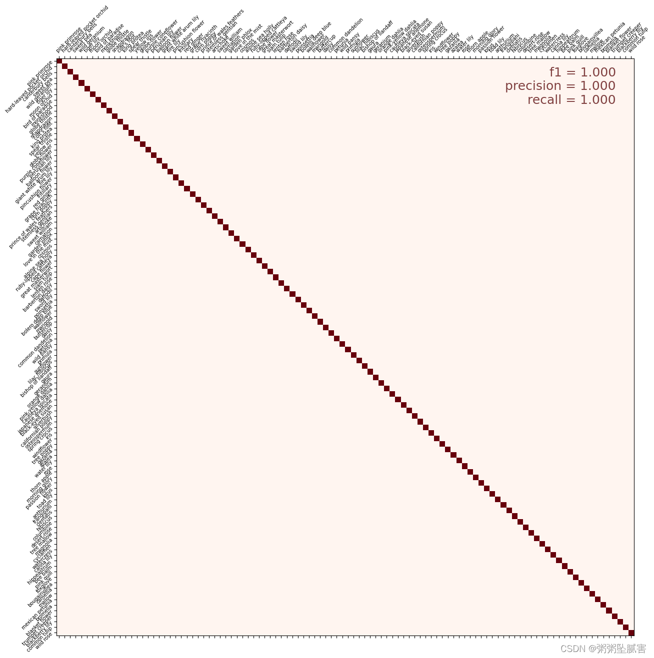

5.4 预测

# 因为我们要分割数据集并分别对图像和ID进行迭代，所以顺序很重要。
test_ds = get_test_dataset(ordered=True) # 测试集# 对测试集进行预测
print('Computing predictions...')
test_images_ds = test_ds.map(lambda image, idnum: image) #测试集的图片
probabilities = model.predict(test_images_ds) # 图片在104个类别上的概率
predictions = np.argmax(probabilities, axis=-1) # 其中最大的概率表示这个图片的预测类别
print(predictions) # 输出预测类别# 生成提交文件
print('Generating submission.csv file...')
test_ids_ds = test_ds.map(lambda image, idnum: idnum).unbatch() #测试集的id
test_ids = next(iter(test_ids_ds.batch(NUM_TEST_IMAGES))).numpy().astype('U') # 准换id的数据类型 # all in one batch# 第一种存储文件方式，不需要pandas
# np.savetxt('submission.csv', np.rec.fromarrays([test_ids, predictions]), fmt=['%s', '%d'], delimiter=',', header='id,label', comments='')
# 第二种存储文件的方式，需要pandas
import pandas as pd
test = pd.DataFrame({"id":test_ids,"label":predictions}) #将id列和label列创建成一个DataFrame
print(test.head) # 输出test的前几行
test.to_csv("submission.csv",index = False) # 生成没有索引的submission.csv，以便提交

Computing predictions...
58/58 [==============================] - 60s 1s/step
[ 78  83 103 ...  49  45 103]
Generating submission.csv file...
<bound method NDFrame.head of              id  label
0     0b9afbdf2     78
1     c37a6f3e9     83
2     00e4f514e    103
3     1c4736dea     28
4     252d840db     67
...         ...    ...
7377  f65475a24     48
7378  9b9c0e574    103
7379  298ade3a4     49
7380  8361401fa     45
7381  e46998f4d    103[7382 rows x 2 columns]>

5.5 验证

dataset = get_validation_dataset()  # 获取验证集
dataset = dataset.unbatch().batch(20)  #将验证集分成大小为20的小批量
batch = iter(dataset) # 将数据集转化为Iterator对象

# 再次运行该单元格以获取下一组图像
images, labels = next(batch) # 获取验证集的下一个批量
probabilities = model.predict(images) # 图片在104个类别上的概率
predictions = np.argmax(probabilities, axis=-1) # 其中最大的概率表示这个图片的预测类别
display_batch_of_images((images, labels), predictions) # 展示一个批量的图片，图片标题为预测标签+预测标签是否正确（OK或NO）
# 举个例子：标题为wild rose（NO->watercress），这个图片实际是豆瓣花，但是预测为野玫瑰，所以它是错的。所以它的标签为 野玫瑰（NO->豆瓣花）

6 结果展示