本文主要是介绍【Intel校企合作课程】淡水质量检测,希望对大家解决编程问题提供一定的参考价值,需要的开发者们随着小编来一起学习吧!
1、项目简介
1.1、问题描述
淡水是我们最重要和最稀缺的自然资源之一,仅占地球总水量的 3%。它几乎触及我们日常生活的方方面面,从饮用、游泳和沐浴到生产食物、电力和我们每天使用的产品。获得安全卫生的供水不仅对人类生活至关重要,而且对正在遭受干旱、污染和气温升高影响的周边生态系统的生存也至关重要。
1.2、预期解决方案:
通过参考英特尔的类似实现方案,预测淡水是否可以安全饮用和被依赖淡水的生态系统所使用,从而可以帮助全球水安全和环境可持续性发展。这里分类准确度和推理时间将作为评分的主要依据。
通过提供的淡水数据集,对数据首先进行数据探索、数据预处理、利用机器学习建立模型,并进行淡水是否可以安全饮用和被依赖淡水的生态系统所使用的质量预测。
1、数据探索:查看数据集规模、数据类型、缺失值情况以及统计性描述。
2、数据预处理:对非数值数据进行转换、处理缺失值和重复值、删除不相关列。
3、利用机器学习建立模型:利用SVC支持向量机分类和XGBClassifier来进行拟合。
1.3、数据集包
你可以在此处下载数据集要求。
1.4、要求
需要使用 英特尔® ONEAPI AI分析工具包。
2、数据探索性分析
2.1、导包和加载数据集
导入项目所需要的包,加载下载好的数据集。
import modin.pandas as pd
import os
os.environ["MODIN_ENGINE"] = "dask"
from modin.config import Engine
Engine.put("dask")import os
import daal4py as d4p
from xgboost import XGBClassifier
import time
import warnings
import pandas
import json
import numpy as np
import seaborn as sns
import matplotlib.pyplot as plt
import matplotlib.colors
import plotly.io as pio
import plotly.express as px
import plotly.graph_objects as go
from plotly.subplots import make_subplots
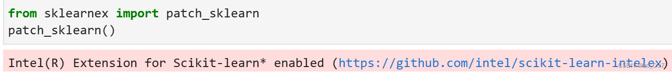
from sklearn.preprocessing import OneHotEncoderfrom sklearnex import patch_sklearn
patch_sklearn()from sklearn.model_selection import train_test_split, StratifiedKFold, GridSearchCV, RandomizedSearchCV
from sklearn.preprocessing import RobustScaler, StandardScaler
from sklearn.metrics import make_scorer, recall_score, precision_score, accuracy_score, roc_auc_score, f1_score
from sklearn.metrics import roc_auc_score, roc_curve, auc, accuracy_score, f1_score
from sklearn.metrics import precision_recall_curve, average_precision_score
from sklearn.svm import SVC
from xgboost import plot_importance
import pickle# 引入可视化函数warnings.filterwarnings('ignore')
pio.renderers.default='notebook' # or 'iframe' or 'colab' or 'jupyterlab'
intel_pal, color=['#0071C5','#FCBB13'], ['#7AB5E1','#FCE7B2']# # 以"layout"为key,后面实例为value创建一个字典
temp=dict(layout=go.Layout(font=dict(family="Franklin Gothic", size=12), height=500, width=1000))# Read data
data = pandas.read_csv('./dataset.csv')
使用modin.pandas库时,将默认的引擎更改为dask。modin.pandas是一个用于处理大型数据集的库,它提供了类似于Pandas的功能,但可以更好地利用分布式计算资源。通过将引擎设置为dask,可以利用Dask库提供的并行计算功能来加速数据处理任务。
2.2、查看数据集
2.2.1、查看数据集前五行
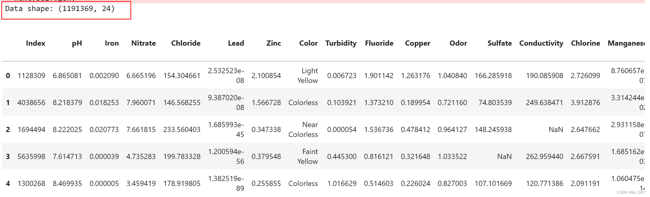
print("Data shape: {}\n".format(data.shape))
display(data.head())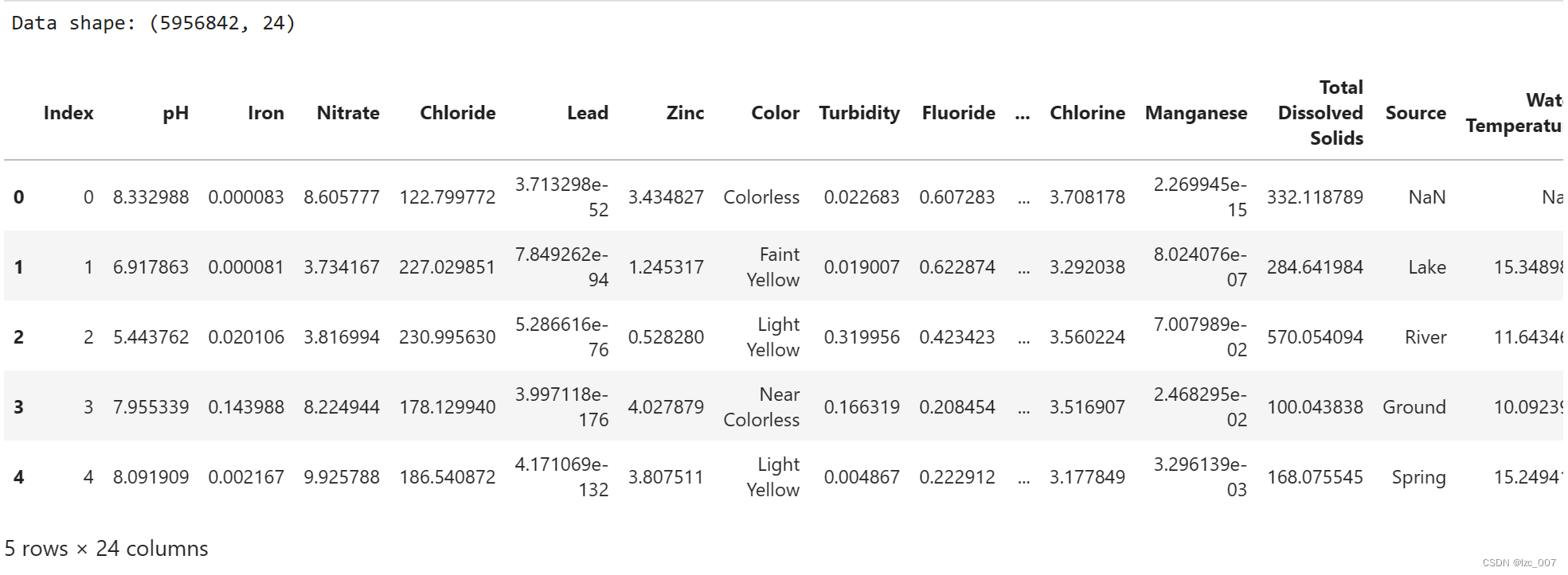
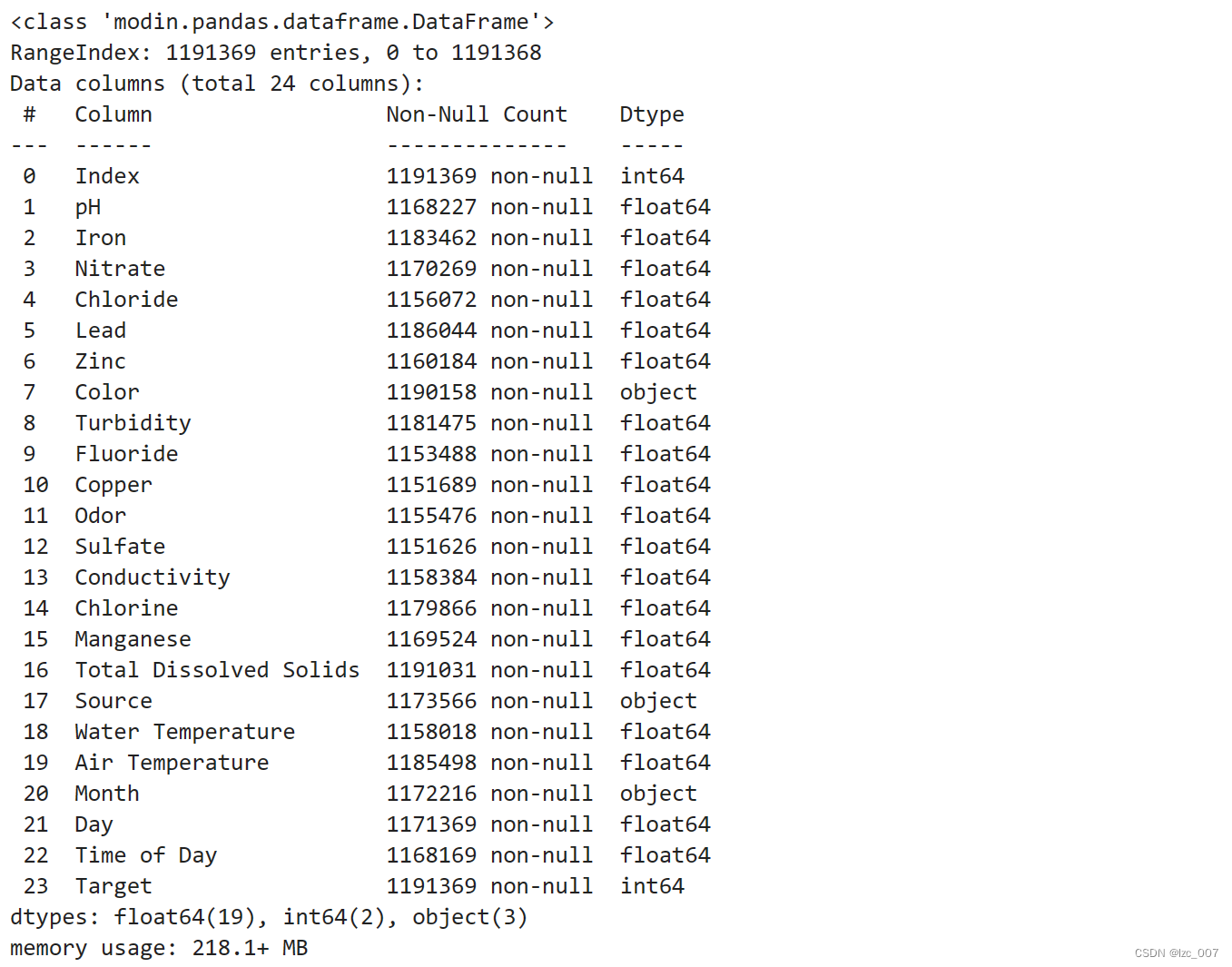
由得到的结果可以看到数据集中共有595684个数据,24个特征列。
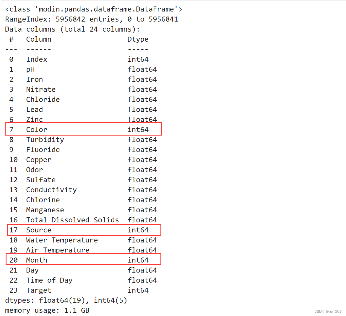
2.2.3、查看数据集基本信息
data=data.infer_objects()
data.info()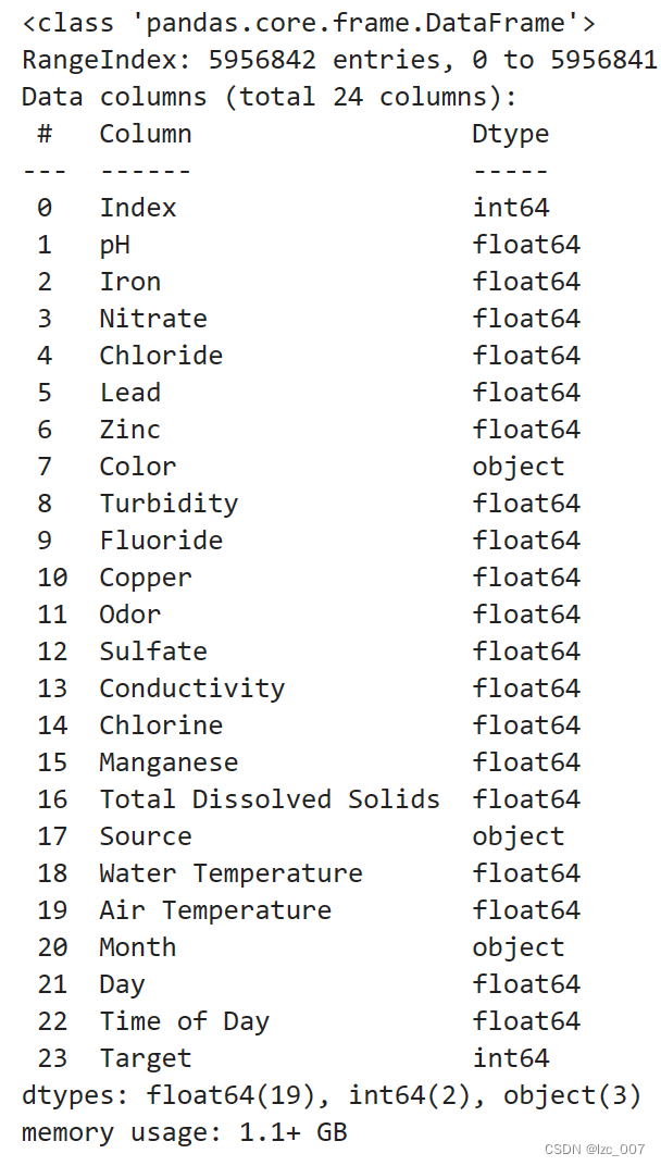
从得到的结果可以看出,数据集中Color、Source和Month是object类型(非数值类型),其余都是数值类型数据。
2.2.4、查看数据中每列的缺失值和重复值
display(data.isna().sum())
missing=data.isna().sum().sum()
duplicates=data.duplicated().sum()
print("\nThere are {:,.0f} missing values in the data.".format(missing))
print("There are {:,.0f} duplicate records in the data.".format(duplicates))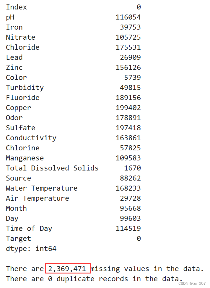
从得到的结果可以看出,数据集共有2369471个缺失值。
2.2.5、查看数据集描述性统计
data.describe()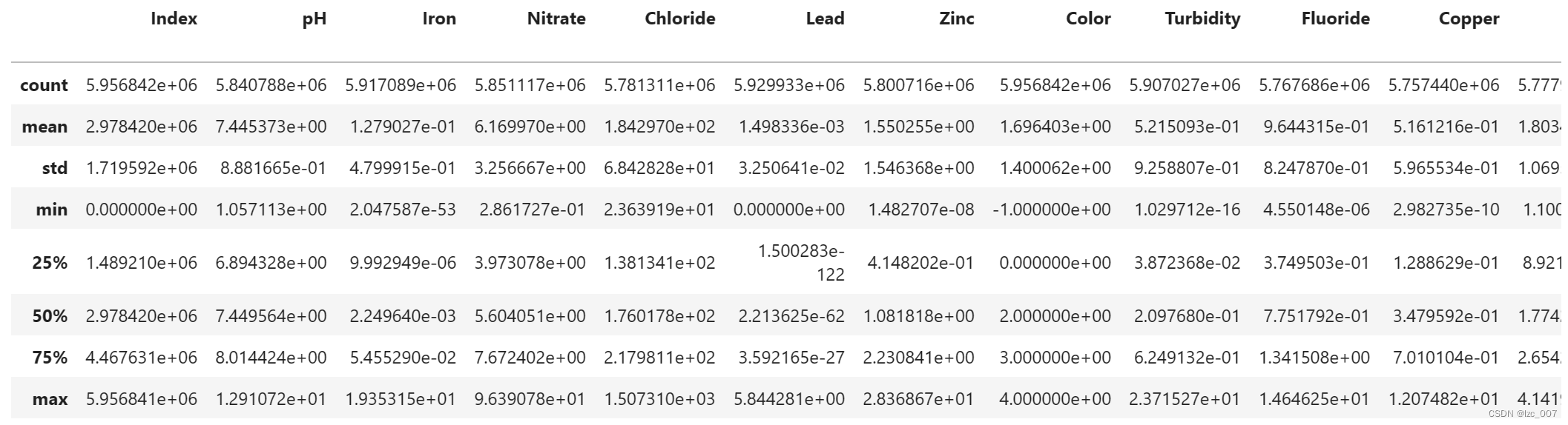
2.3、数据可视化分析
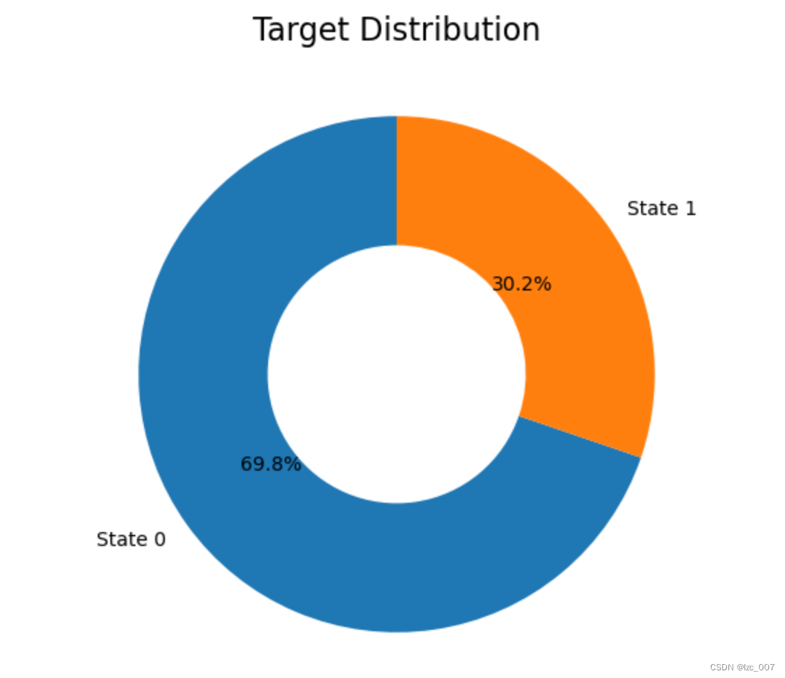
2.3.1、查看正常和异常类的比例
#查看正常和异常类的数量
print('正常数据数量为{}' . format( len(data [data['Target']==0])))
print('异常数据数量为{}' .format(len(data[data['Target']==1])))
print('比例为{}:1'.format(int(len(data[data[ 'Target']==0])/len(data[data['Target']==1]))))import matplotlib.pyplot as pltdef plot_target(target_col):tmp=data[target_col].value_counts(normalize=True)target = tmp.rename(index={1:'Class 1',0:'Class 0'})wedgeprops = {'width':0.5, 'linewidth':10}plt.figure(figsize=(6,6))plt.pie(list(tmp), labels=target.index,startangle=90, autopct='%1.1f%%',wedgeprops=wedgeprops)plt.title('Label Distribution', fontsize=16)plt.show() plot_target(target_col='Target')


数据集中正常数据(即可以饮用的淡水,Target=0)和异常数据的比例约为2:1,比较正常,故后续不需要对数据集进行额外的数据平衡操作,饼状图如上图所示。
2.3.2、相关性分析
# 相关性分析
bar = data.corr()['Target'].abs().sort_values(ascending=False)[1:]plt.bar(bar.index, bar, width=0.5)
# 设置figsize的大小
pos_list = np.arange(len(data.columns))
params = {'figure.figsize': '20, 18'
}·
plt.rcParams.update(params)
plt.xticks(bar.index, bar.index, rotation=-60, fontsize=10)
plt.show()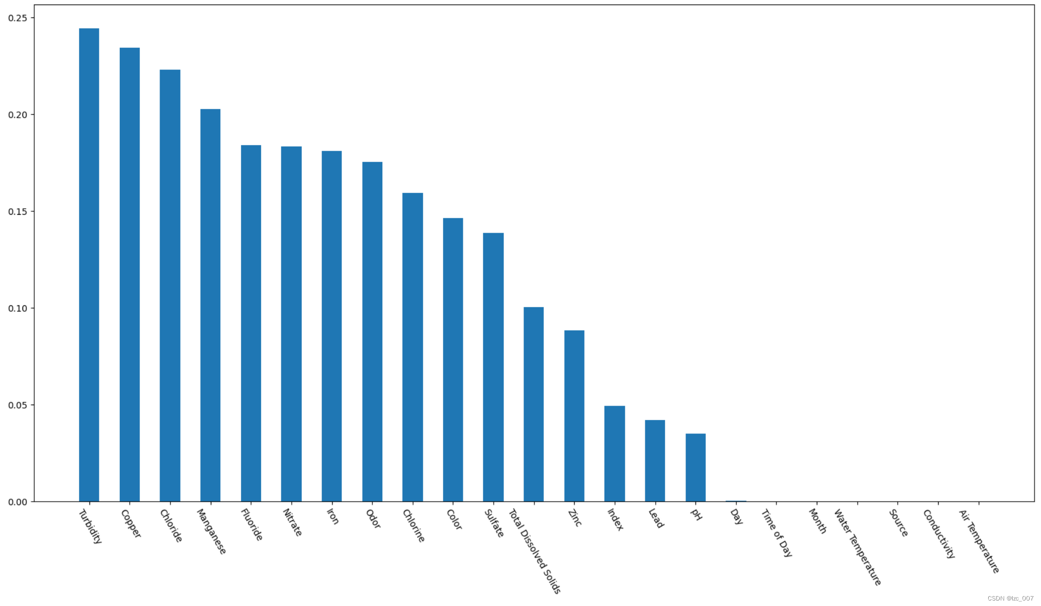
从中可以看出,数据集中的'Index', 'Day', 'Time of Day', 'Month', 'Water Temperature', 'Source', 'Conductivity', 'Air Temperature'与Target列的相关性不大。
2.3.3、箱形图
# 获取数据集中的所有列名
columns = data.columns# 计算行数和列数
num_columns = len(columns)
num_rows = (num_columns + 2) // 3  # 向上取整除法# 逐个绘制每个特征的箱形图
plt.figure(figsize=(12, 4*num_rows))
for i, column in enumerate(columns):plt.subplot(num_rows, 3, i + 1)sns.boxplot(x=data[column])plt.title('Boxplot of {}'.format(column))plt.xlabel(column)
plt.tight_layout()
plt.show()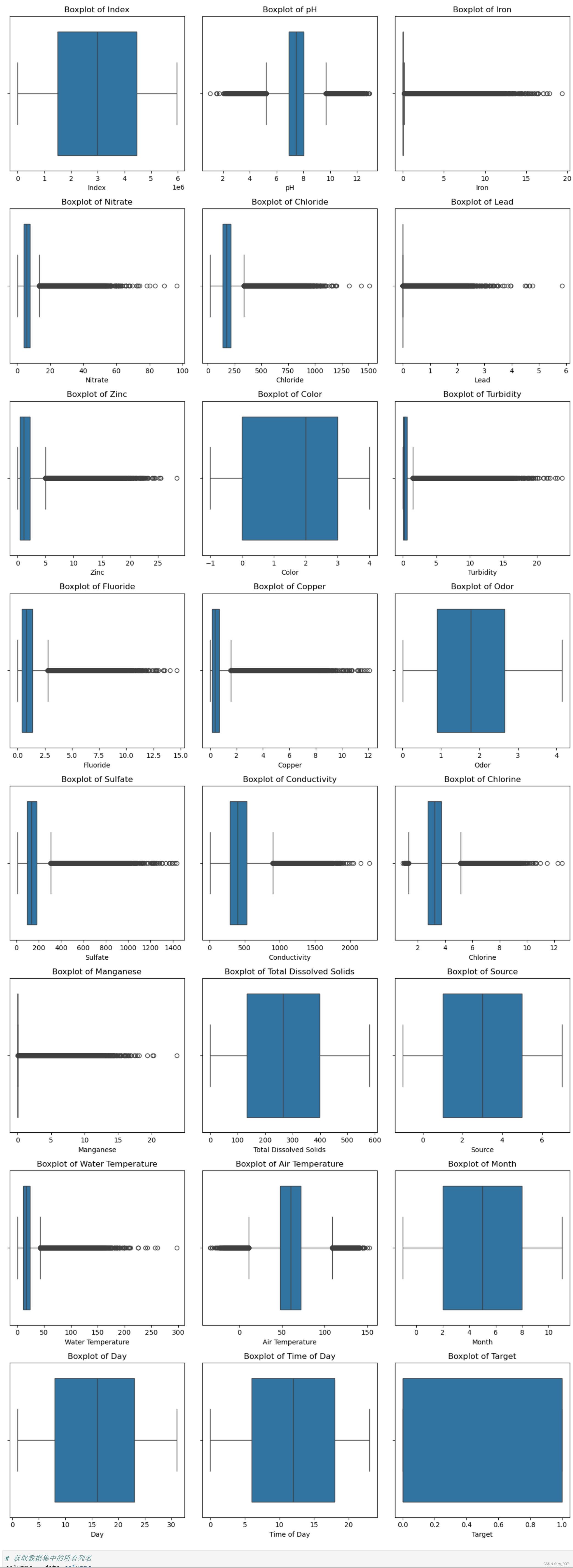
通过箱形图查看各个属性分散情况。
2.3.4、直方图
# 划分类别特征, 数值特征
cat_cols, float_cols = [], ['Target']
for col in data.columns:if data[col].value_counts().count() < 50:cat_cols.append(col)else:float_cols.append(col)
print('离散特征:', cat_cols)
print('连续特征:', float_cols)
data[float_cols].hist(bins=50,figsize=(16,12))
通过直方图的形式查看连续性数据的分布,只有类似于正态分布的数据分布才是符合现实规律的数据,并且这有利于模型的训练。既有符合正态分布的,也有比较不符合的,后续需要对不符合正态分布的特征数据进行数据转换。
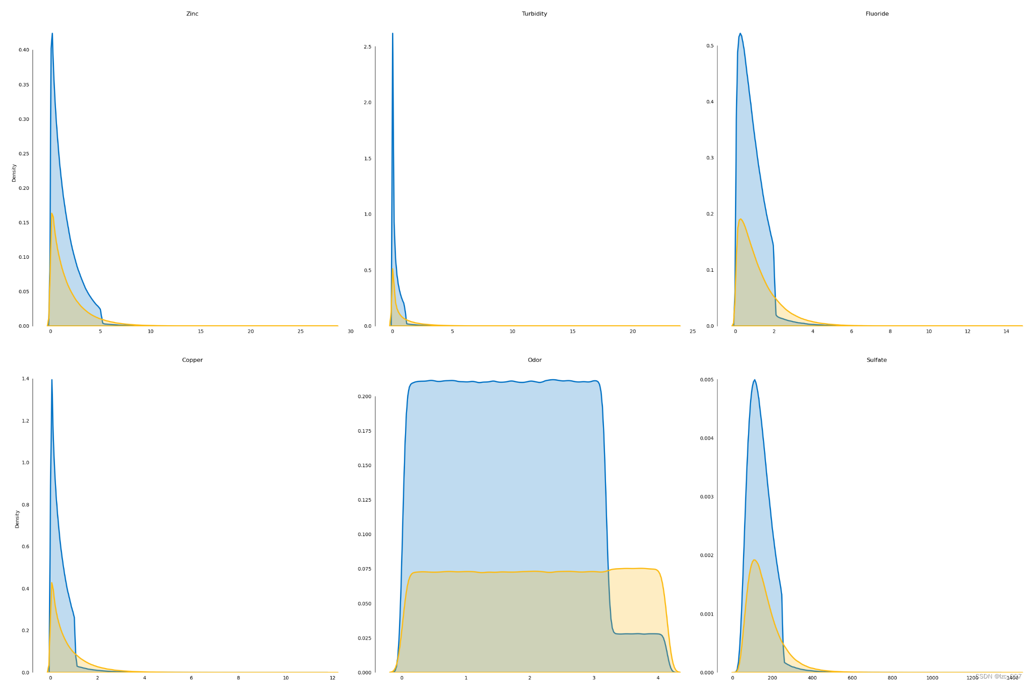
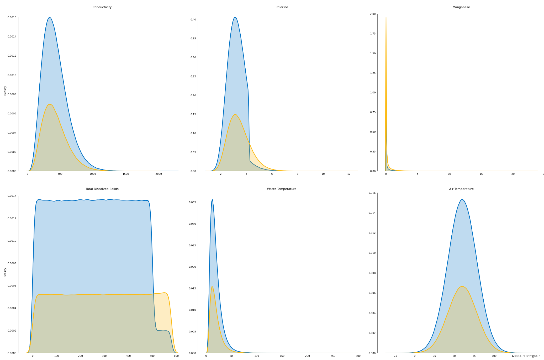
2.3.5、密度图
# 密度图
l = len(float_cols)
plot_df=data[float_cols]
fig, ax = plt.subplots(10,3, figsize=(30,100))
fig.suptitle('Distribution of Numerical Variables',fontsize=32)
row=0
col=[0,1,2]*10
for i, column in enumerate(plot_df.columns[1:]):if (i!=0)&(i%3==0):row+=1sns.kdeplot(x=column, hue='Target', palette=intel_pal[::-1], hue_order=[1,0], label=['State 1','State 0'], data=plot_df, fill=True, linewidth=2.5, legend=False, ax=ax[row,col[i]])ax[row,col[i]].tick_params(left=False, bottom=False)ax[row,col[i]].set(title='\n\n{}'.format(column), xlabel='', ylabel=('Density' if i%3==0 else ''))handles, _ = ax[0,0].get_legend_handles_labels()
fig.legend(labels=['State 1','State 0'], handles=reversed(handles))
sns.despine(bottom=True, trim=True)
plt.tight_layout()# 显示图形
plt.show()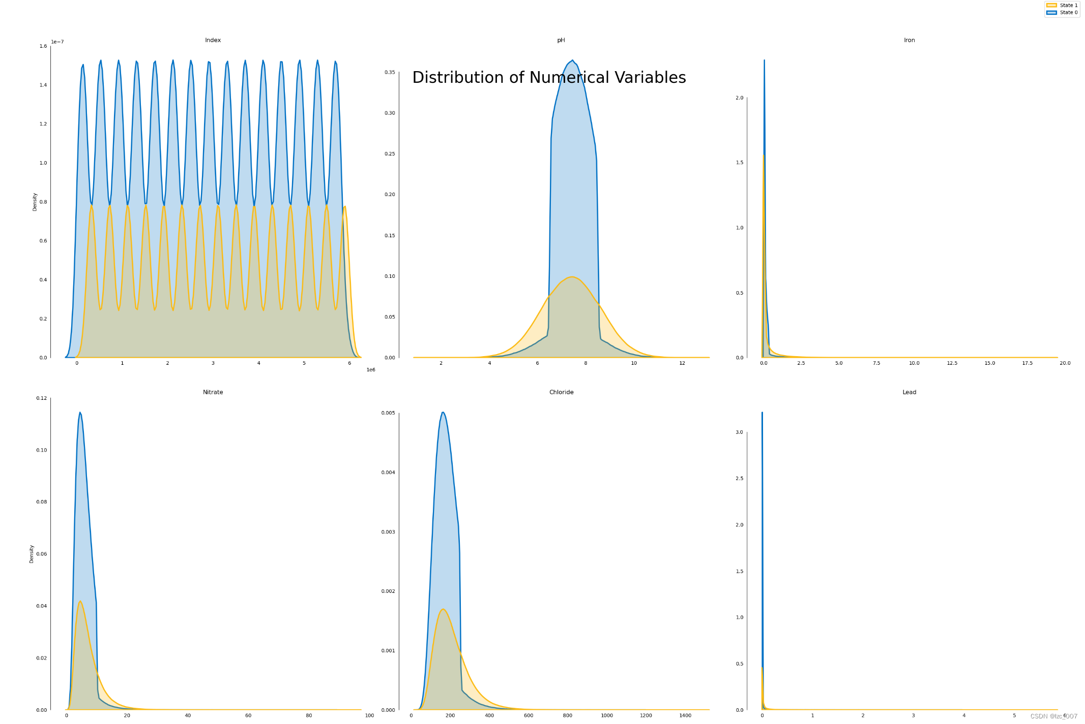
2.3.6、热力图
# 计算相关系数矩阵
corr_matrix = data.corr(method='spearman')# 设置图形尺寸和分辨率
fig, ax = plt.subplots(figsize=(30, 20), dpi=128)# 绘制热力图
heatmap = sns.heatmap(corr_matrix, annot=True, square=True, ax=ax)# 添加标题
plt.title('Correlation Heatmap', fontsize=16)# 显示图形
plt.show()

3、数据预处理
3.1、将非数值类型数据转化为数值类型
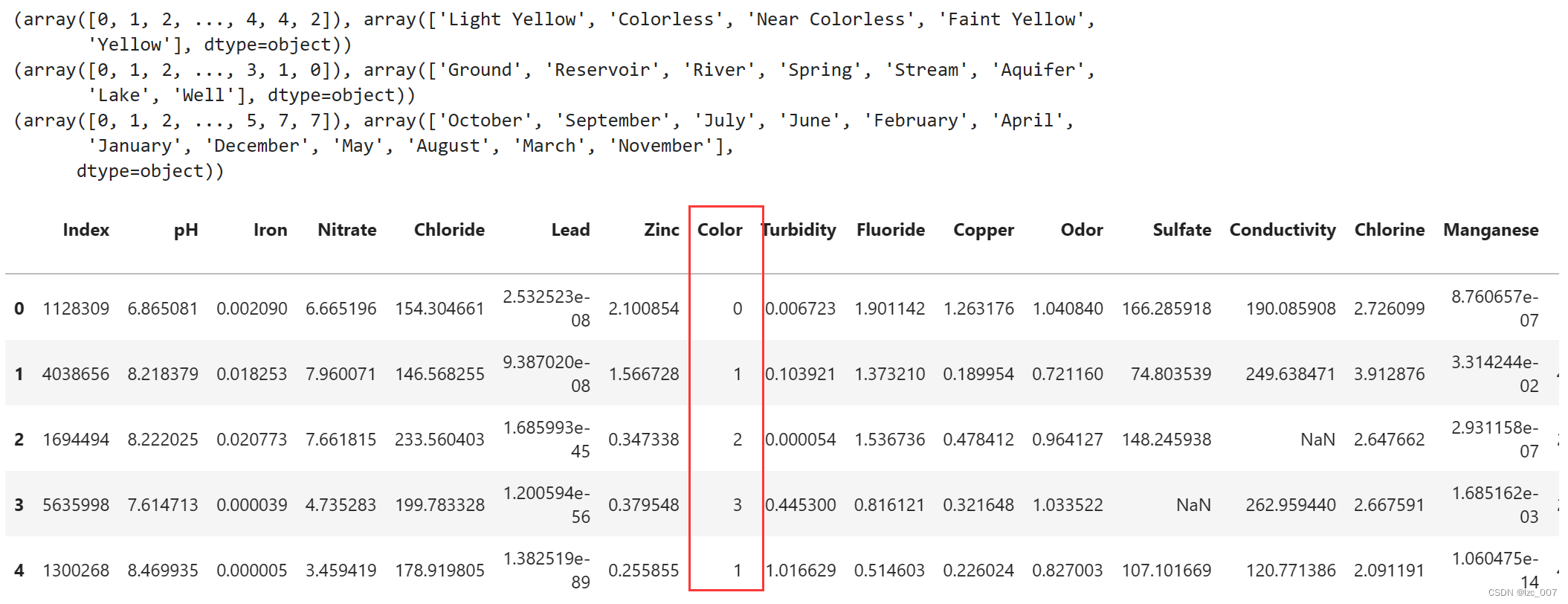
factor = pd.factorize(data['Color'])
print(factor)
data.Color = factor[0]
factor = pd.factorize(data['Source'])
print(factor)
data.Source = factor[0]
factor = pd.factorize(data['Month'])
print(factor)
data.Month = factor[0]
display(data.head())data.info
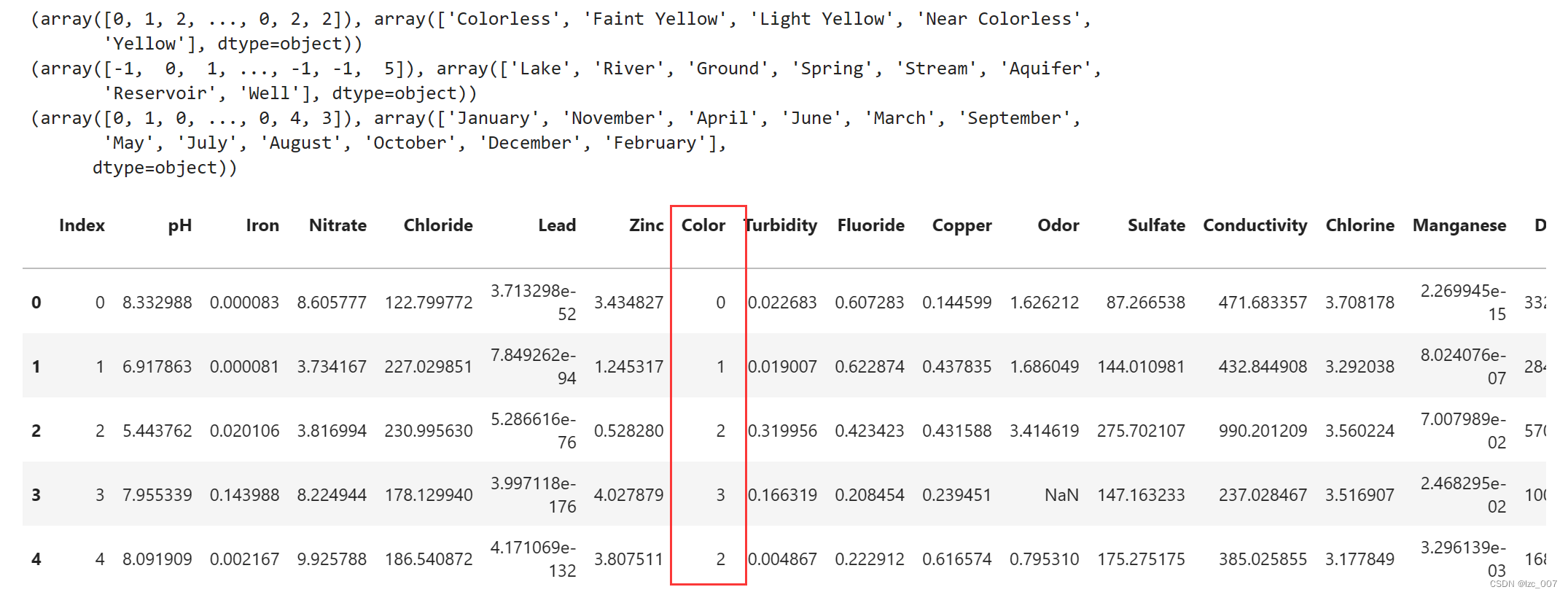
将数据集中的非数值类型数据,即'Color'、'Source'和'Month'列进行因子化处理,转换成数值类型。因子化是一种将分类变量转换为数值表示的方法,通常用于机器学习模型的输入。
从结果可以看到将三列object类型数据转换成了Int类型数据。
3.2、处理缺失值和重复值
#所有特征值为空的样本以0填充,删除重复值
data = data.fillna(0)
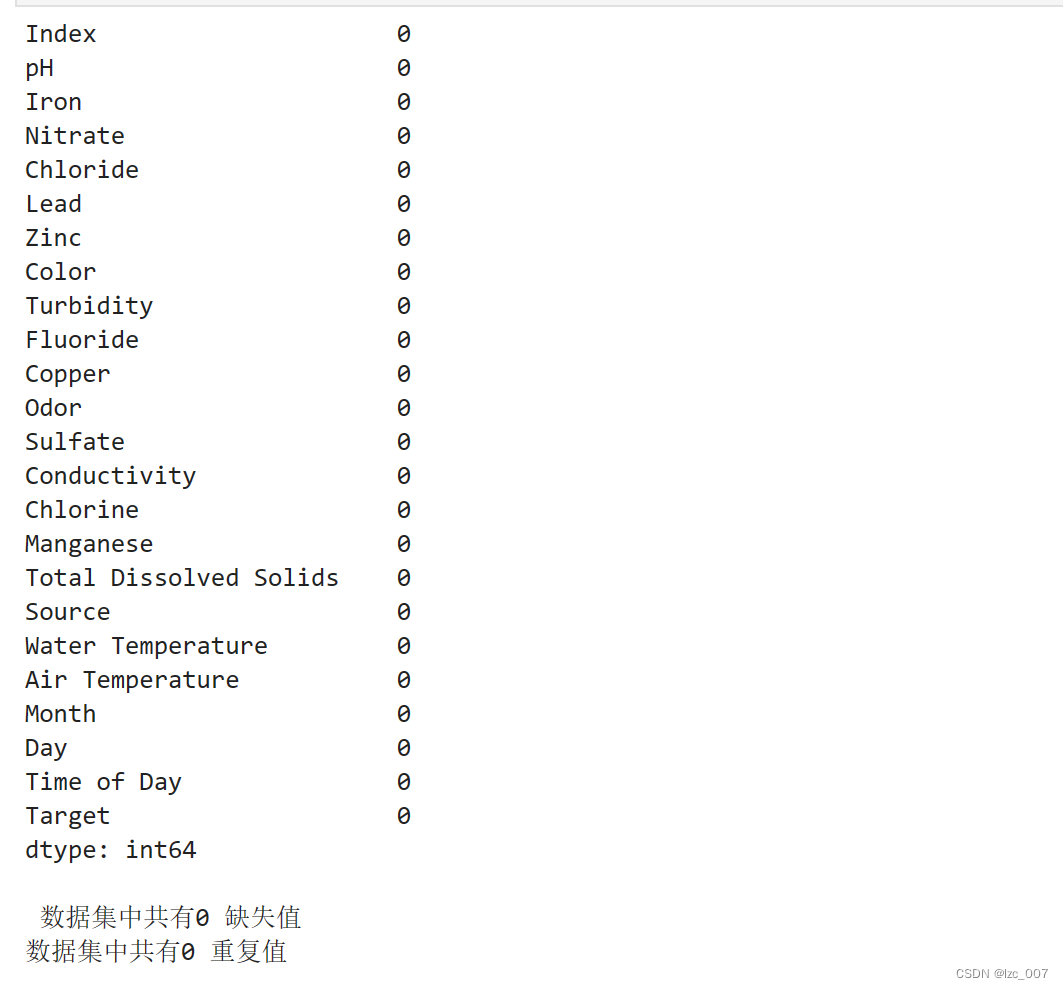
data = data.drop_duplicates()display(data.isna().sum())
missing = data.isna().sum().sum()
duplicates = data.duplicated().sum()
print("\n 数据集中共有{:,.0f} 缺失值 ".format(missing))
print("数据集中共有{:,.0f} 重复值 ".format(duplicates))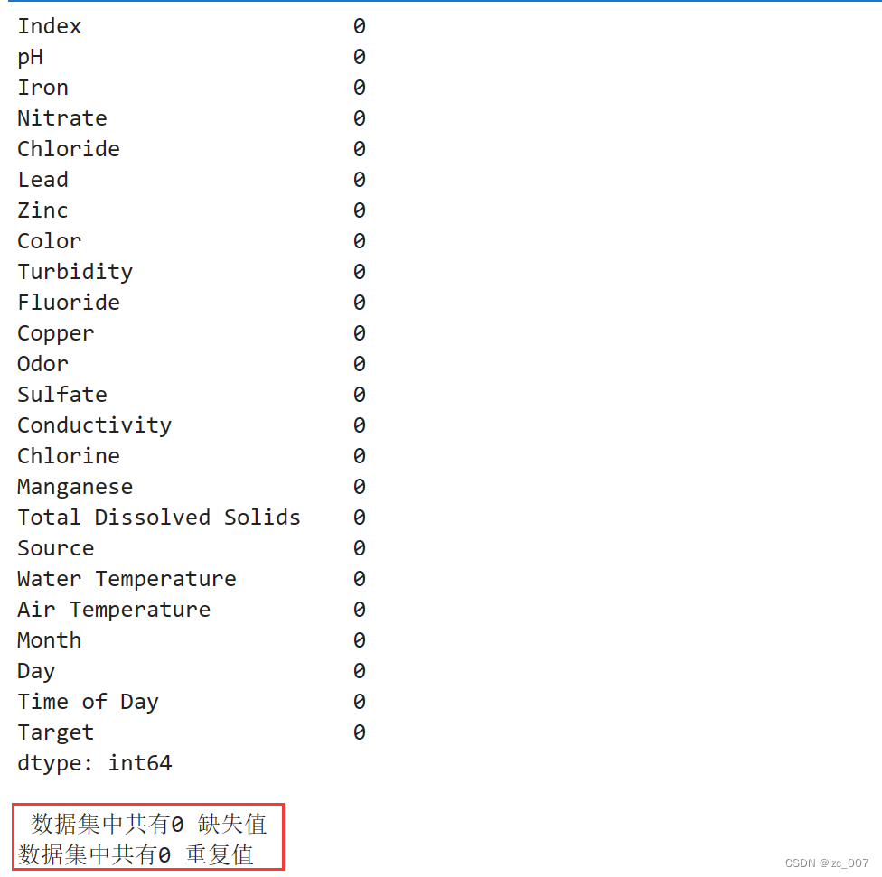
从得到的结果可以看出,处理过后的数据集没有缺失值和重复值。
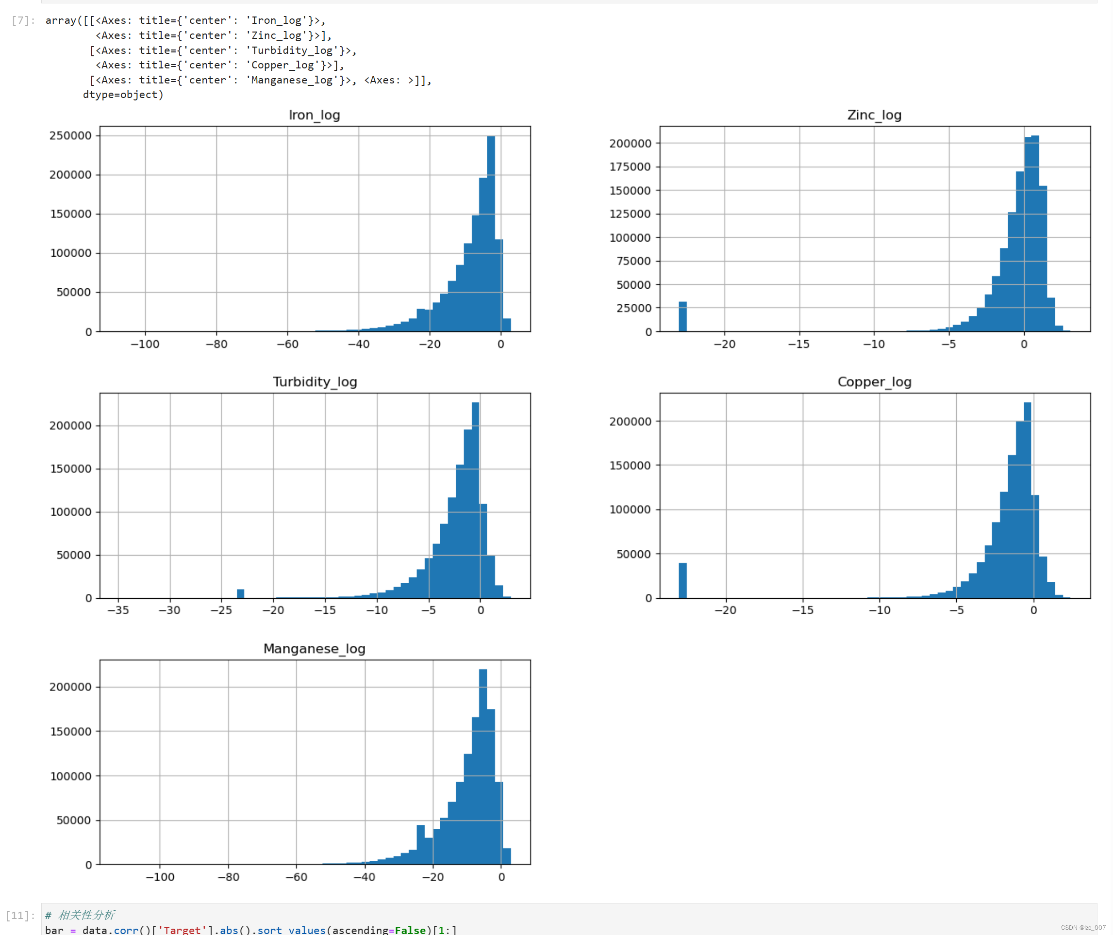
3.3、针对不规则分布的变量进行非线性变换(log)
# 针对不规则分布的变量进行非线性变换,一般进行log
log_col = ['Iron', 'Zinc', 'Turbidity', 'Copper', 'Manganese']
show_col = []
for col in log_col:data[col + '_log'] = np.log(data[col])show_col.append(col + '_log')# 特殊地,由于Lead变量0值占据了一定比例,此处特殊处理Lead变量
excep_col = ['Lead']
spec_val = {}
# 先将0元素替换为非0最小值,再进行log变换
for col in excep_col:spec_val[col] = data.loc[(data[col] != 0.0), col].min()data.loc[(data[col] == 0.0), col] = data.loc[(data[col] != 0.0), col].min()data[col + '_log'] = np.log(data[col])show_col.append(col + '_log')data[show_col].hist(bins=50,figsize=(16,12))
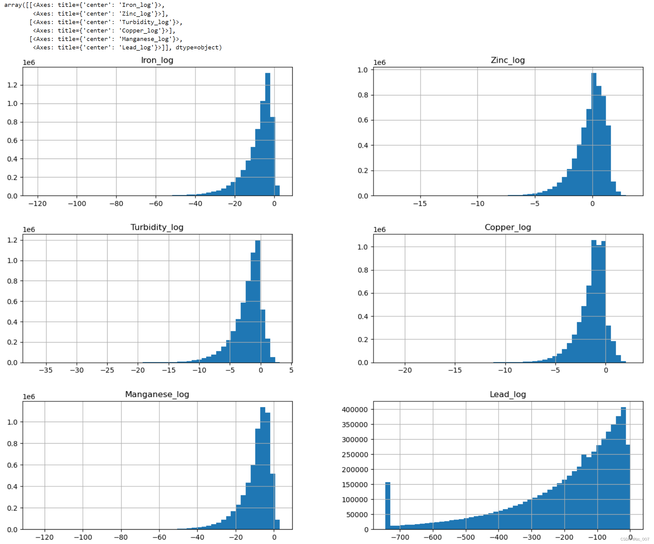
从得到结果可以看出,经过变换过后的数据已经符合正态分布。
3.4、删除相关性不大的特征
#后续的特征数据的相关性都比较差,所以这里采取的做法为删除相关特征以及对应的列数据
data = data.drop(columns=['Index', 'Day', 'Time of Day', 'Month', 'Water Temperature', 'Source', 'Conductivity', 'Air Temperature'])
由相关性分析所得到的图可知,后续的特征数据的相关性都比较差,所以这里采取的做法为删除相关特征以及对应的列数据。
3.5、偏差值处理
from scipy.stats import pearsonrvariables = data.columns
data = datavar = data.var()
numeric = data.columns
data = data.fillna(0)
for i in range(0, len(var) - 1):if var[i] <= 0.1:  # 方差大于10%print(variables[i])data = data.drop(numeric[i], axis=1)
variables = data.columnsfor i in range(0, len(variables)):x = data[variables[i]]y = data[variables[-1]]if pearsonr(x, y)[1] > 0.05:print(variables[i])data = data.drop(variables[i], axis=1)variables = data.columns
print(variables)
print(len(variables)) 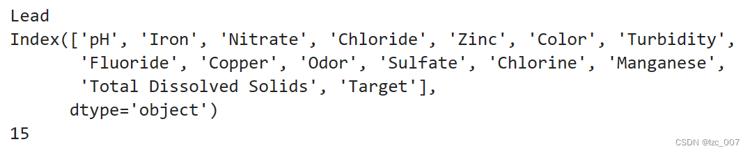
对偏差值进行处理,通过检查皮尔逊相关系数与缺失值比例是否大于20%,数值型特征方差是否小于0.1来进行删除特征操作。
最后剩下的特征如上所示。
到这里,数据的探索性分析和预处理基本已经完成,接下来就正式开始模型的拟合。
4、模型拟合
from sklearn.model_selection import train_test_split, StratifiedKFold, GridSearchCV, RandomizedSearchCV
from sklearn.preprocessing import RobustScaler
from sklearn.metrics import roc_auc_score, roc_curve, auc, accuracy_score, f1_score
from sklearn.metrics import precision_recall_curve, average_precision_score
from sklearn.svm import SVC
import warnings
warnings.filterwarnings("ignore")
import plotly.io as pio
warnings.filterwarnings('ignore')
pio.renderers.default='jupyterlab' # or 'iframe' or 'colab' or 'jupyterlab'
intel_pal, color=['#0071C5','#FCBB13'], ['#7AB5E1','#FCE7B2']# # 以"layout"为key,后面实例为value创建一个字典
temp=dict(layout=go.Layout(font=dict(family="Franklin Gothic", size=12), height=500, width=1000))def prepare_train_test_data(data, target_col, test_size):scaler = RobustScaler()   X = data.drop(target_col, axis=1)y = data[target_col]X_train, X_test, y_train, y_test = train_test_split(X, y, test_size=test_size, random_state=21)X_train_scaled = scaler.fit_transform(X_train)X_test_scaled = scaler.transform(X_test)print("Train Shape: {}".format(X_train_scaled.shape))print("Test Shape: {}".format(X_test_scaled.shape))return X_train_scaled, X_test_scaled, y_train, y_testdef plot_model_res(model_name, y_test, y_prob):intel_pal=['#0071C5','#FCBB13']color=['#7AB5E1','#FCE7B2']fpr, tpr, _ = roc_curve(y_test, y_prob)roc_auc = auc(fpr,tpr)precision, recall, _ = precision_recall_curve(y_test, y_prob)auprc = average_precision_score(y_test, y_prob)fig = make_subplots(rows=1, cols=2, shared_yaxes=True, subplot_titles=['Receiver Operating Characteristic<br>(ROC) Curve','Precision-Recall Curve<br>AUPRC = {:.3f}'.format(auprc)])fig.add_trace(go.Scatter(x=np.linspace(0,1,11), y=np.linspace(0,1,11), name='Baseline',mode='lines',legendgroup=1,line=dict(color="Black", width=1, dash="dot")), row=1,col=1)    fig.add_trace(go.Scatter(x=fpr, y=tpr, line=dict(color=intel_pal[0], width=3), hovertemplate = 'True positive rate = %{y:.3f}, False positive rate = %{x:.3f}',name='AUC = {:.4f}'.format(roc_auc),legendgroup=1), row=1,col=1)fig.add_trace(go.Scatter(x=recall, y=precision, line=dict(color=intel_pal[0], width=3), hovertemplate = 'Precision = %{y:.3f}, Recall = %{x:.3f}',name='AUPRC = {:.4f}'.format(auprc),showlegend=False), row=1,col=2)fig.update_layout(template=temp, title="{} ROC and Precision-Recall Curves".format(model_name), hovermode="x unified", width=900,height=500,xaxis1_title='False Positive Rate (1 - Specificity)',yaxis1_title='True Positive Rate (Sensitivity)',xaxis2_title='Recall (Sensitivity)',yaxis2_title='Precision (PPV)',legend=dict(orientation='v', y=.07, x=.45, xanchor="right",bordercolor="black", borderwidth=.5))fig.show()def plot_distribution(y_prob): plot_df=pd.DataFrame.from_dict({'State 0':(len(y_prob[y_prob<=0.5])/len(y_prob))*100, 'State 1':(len(y_prob[y_prob>0.5])/len(y_prob))*100}, orient='index', columns=['pct'])fig=go.Figure()fig.add_trace(go.Pie(labels=plot_df.index, values=plot_df.pct, hole=.45, text=plot_df.index, sort=False, showlegend=False,marker=dict(colors=color,line=dict(color=intel_pal,width=2.5)),hovertemplate = "%{label}: <b>%{value:.2f}%</b><extra></extra>"))fig.update_layout(template=temp, title='Predicted Target Distribution',width=700,height=450,uniformtext_minsize=15, uniformtext_mode='hide')fig.show()
利用Intel AI Analytics Toolkit中Machine Learning模块中的intel extension for Scikit-learn进行模型拟合。
XGBClassifier是一个功能强大的分类器,它通过集成多个CART回归树来提高预测的准确性。
import time
import daal4py as d4p
## Prepare Train and Test datasets ##
print("Preparing Train and Test datasets")
X_train, X_test, y_train, y_test = prepare_train_test_data(data=data,target_col='Target', test_size=.25)## Initialize XGBoost model ##
ratio = float(np.sum(y_train == 0)) / np.sum(y_train == 1)
parameters = {'scale_pos_weight': ratio.round(2), 'tree_method': 'hist','random_state': 21}
xgb_model = XGBClassifier(**parameters)## Tune hyperparameters ##
strat_kfold = StratifiedKFold(n_splits=3, shuffle=True, random_state=21)
print("\nTuning hyperparameters..")
grid = {'min_child_weight': [1, 5, 10],'gamma': [0.5, 1, 1.5, 2, 5],'max_depth': [3, 4, 5],}grid_search = GridSearchCV(xgb_model, param_grid=grid, cv=strat_kfold, scoring='roc_auc', verbose=1, n_jobs=-1)
start_time = time.time()
grid_search.fit(X_train, y_train)
end_time = time.time()
# 计算模型拟合时间
fit_time = end_time - start_time
print("模型拟合时间:{:.2f}秒".format(fit_time))print("Done!\nBest hyperparameters:", grid_search.best_params_)
print("Best cross-validation AUC: {:.4f}".format(grid_search.best_score_))## Convert XGB model to daal4py ##
xgb = grid_search.best_estimator_
daal_model = d4p.get_gbt_model_from_xgboost(xgb.get_booster())## Calculate predictions ##
daal_prob = d4p.gbt_classification_prediction(nClasses=2,resultsToEvaluate="computeClassLabels|computeClassProbabilities",fptype='float').compute(X_test, daal_model).probabilities # or .predictions
xgb_pred = pd.Series(np.where(daal_prob[:,1]>.5, 1, 0), name='Target')
xgb_auc = roc_auc_score(y_test, daal_prob[:,1])
xgb_f1 = f1_score(y_test, xgb_pred)  ## Plot model results ##
print("\nTest F1 Accuracy: {:.2f}%, AUC: {:.5f}".format(xgb_f1*100, xgb_auc))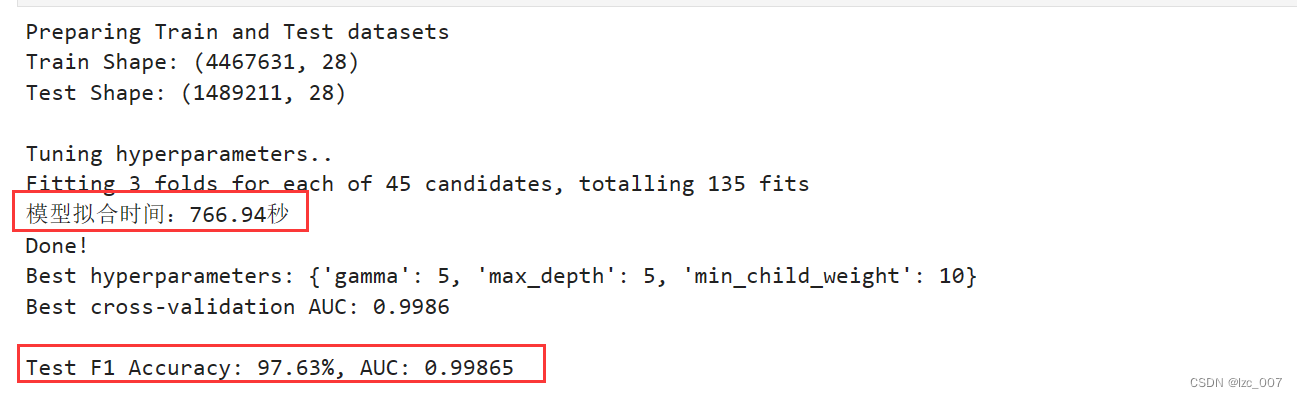
模型拟合得到的F1分数为97%,准确度0.99。
保存模型以便后续预测的使用。
plot_model_res(model_name='XGBoost', y_test=y_test, y_prob=daal_prob[:, 1])
plot_distribution(daal_prob[:,1])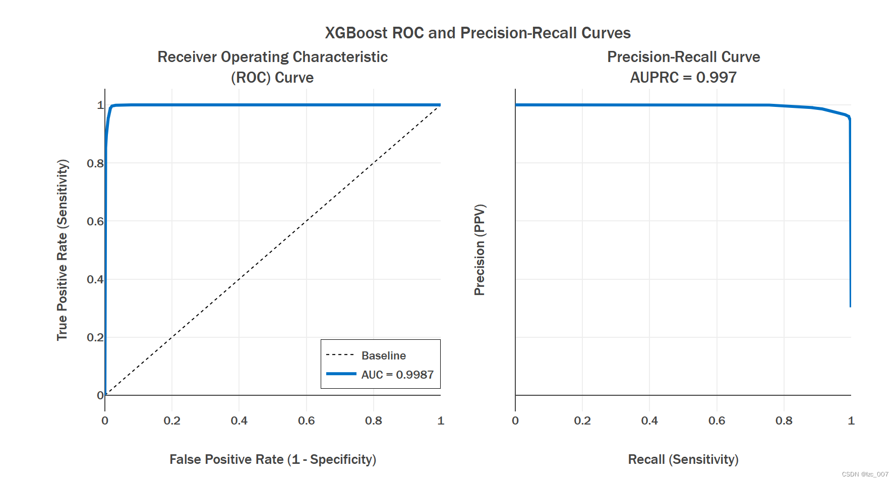
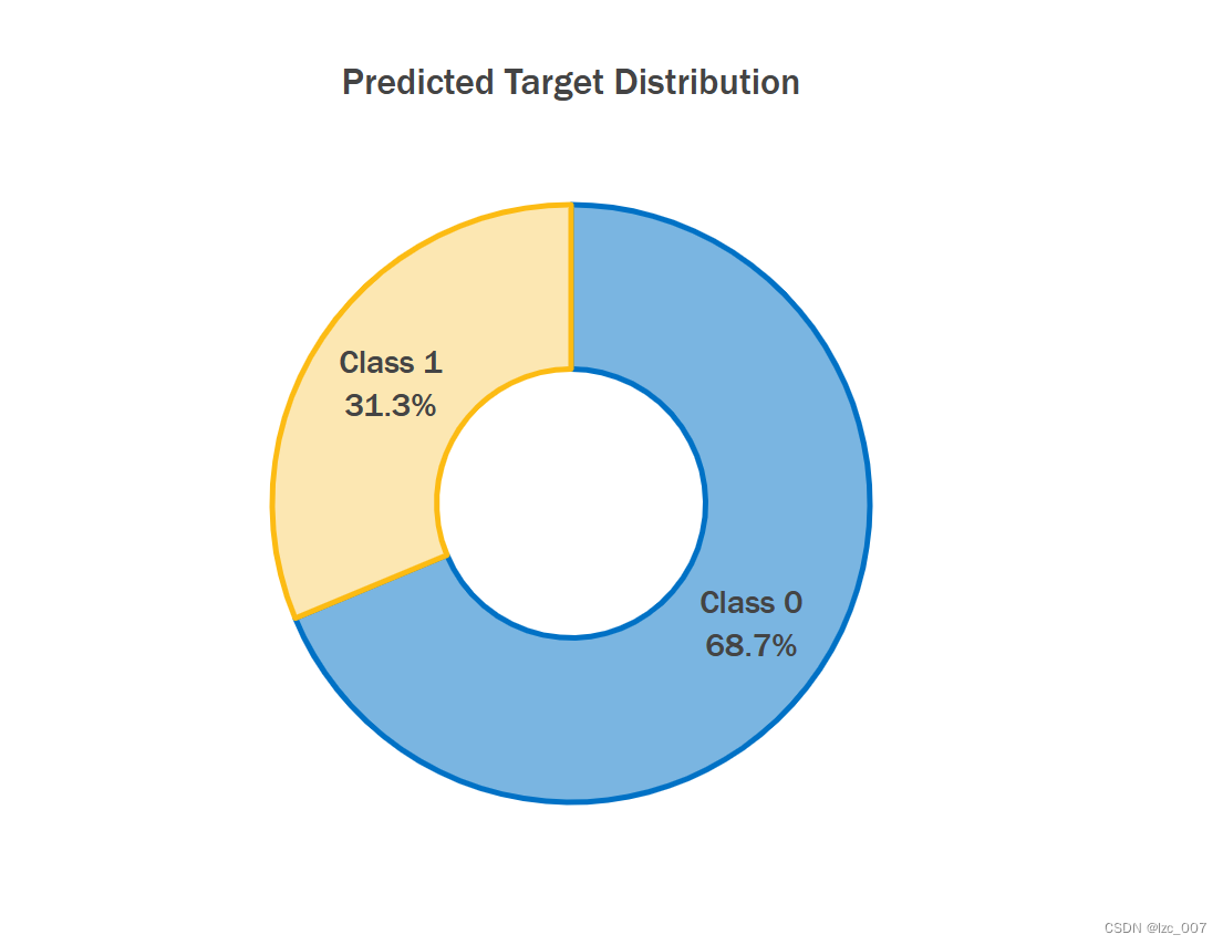
print('预测类别为正常的数量为:{:d}'.format(len(daal_prob[:,1][daal_prob[:,1]<=0.5])))
print('预测类别为异常的数量为:{:d}'.format(len(daal_prob[:,1][daal_prob[:,1]>=0.5])))
5、模型预测
5.1、数据预处理
由于项目要求需要对给定的测试集进行预测,并计算推理时间和F1分数,测试集的数据探索性分析和预处理与前面类似,故只用给出部分结果展示。
转换非数值类型数据为数值型。

5.2、使用保存的模型预测
import joblib# 1. 加载之前保存的模型
loaded_model = joblib.load('xgb_model.pkl')import daal4py as d4ptarget_col = 'Target'# 提取特征列和目标列
features = data.drop(columns=[target_col])
target = data[target_col]# 使用 daal4py 方法对新数据集进行预测
start_time = time.time()
daal_predictions = d4p.gbt_classification_prediction(nClasses=2,resultsToEvaluate="computeClassLabels|computeClassProbabilities",fptype='float').compute(features, loaded_model).probabilities
end_time = time.time()# 计算推理时间
inference_time = end_time - start_time
print("推理时间:{:.2f}秒".format(inference_time))from sklearn.metrics import f1_scoretrue_labels = data['Target']# 将概率转换为类别
predicted_labels = np.where(daal_predictions[:, 1] > 0.5, 1, 0)# 计算 F1 分数
f1 = f1_score(true_labels, predicted_labels)
print("F1 分数:f1")# 打印预测结果
print("预测结果:", daal_predictions)
最后预测的结果所需要的推理时间为6.78秒,F1分数约为0.92。
6、总结
6.1、oneAPI的使用
Intel Extension for PyTorch
"Intel Extension for PyTorch" 是英特尔为 PyTorch 框架提供的一组扩展,目的是优化 PyTorch 在英特尔硬件上的性能。这个扩展旨在充分发挥英特尔处理器的潜力,提高深度学习模型的训练和推断效率。
Intel Extension for Scikit-learn
Intel Extension for Scikit-learn 是一种优化了的 Scikit-learn 库,旨在提高在 Intel 架构上运行时的性能和效率。它利用了 Intel 架构的硬件特性和优化技术,如 Intel MKL(Math Kernel Library)、Intel TBB(Threading Building Blocks)等,从而加速机器学习算法的执行过程。
通过 Intel Extension for Scikit-learn,用户可以在保持 Scikit-learn API 不变的情况下,享受更快的模型训练和预测速度。该扩展库提供了针对常见机器学习任务的优化实现,如线性模型、支持向量机、随机森林等。同时,它还支持在多核处理器上的并行计算,提高了算法的并行度和可扩展性。
总的来说,Intel Extension for Scikit-learn 提供了一种简单而有效的方式来利用 Intel 架构的性能优势,加速 Scikit-learn 中的机器学习任务,从而提高了数据科学工作流程的效率和生产力。
XGBClassifier
XGBClassifier是一种基于梯度提升树(Gradient Boosting Tree)的分类器,它是XGBoost(eXtreme Gradient Boosting)库中的一个类。XGBoost是一种高效的、可扩展的机器学习算法,广泛用于数据科学、机器学习和大规模数据分析任务中。
XGBClassifier的工作原理是通过迭代地训练多个决策树模型来对数据进行分类。在每一次迭代中,它会根据前一轮迭代的结果来调整模型参数,以减小当前轮次的错误。这种迭代的过程会持续进行多个轮次,直到达到设定的停止条件。
6.2、项目的总结
通过本次校企合作课程,我了解到了intel下的oneAPI在机器学习与数据挖掘领域的应用,通过作业实际体验到了intel AI Analytics Toolkit工具实际对于问题解决的提升。
通过该项目,实现了一个完整的分类模型开发流程,从数据准备、模型训练到模型评估和预测。借助XGBoost和daal4py等库,能够高效地构建和部署机器学习模型。通过可视化和指标评估,能够全面地了解模型的性能和预测效果。在处理新数据时,能够灵活地使用保存的模型进行预测,并得到所需的结果。
综上所述,该项目提供了一个实践机器学习项目的示例,涵盖了数据处理、模型训练、评估和预测等多个方面,为理解和应用机器学习提供了有益的参考。
这篇关于【Intel校企合作课程】淡水质量检测的文章就介绍到这儿,希望我们推荐的文章对编程师们有所帮助!