Python环境下基于1D-CNN、2D-CNN和LSTM的一维信号分类

本文主要是介绍Python环境下基于1D-CNN、2D-CNN和LSTM的一维信号分类，希望对大家解决编程问题提供一定的参考价值，需要的开发者们随着小编来一起学习吧！

以简单的西储大学轴承数据集为例，随便你下载几个信号玩耍吧，我选了10个信号，分别求为正常状态，内圈（轻、中和重度损伤），外圈（轻、中和重度损伤），滚动体（轻、中和重度损伤）。

首先导入相关模块

import scipy.io
import numpy as np
from sklearn.model_selection import train_test_split, KFold
from sklearn.metrics import confusion_matrix
import tensorflow as tf
from tensorflow.keras import layers, models
import matplotlib.pyplot as plt
import seaborn as sns
import pandas as pd

定义一个导入数据函数

def ImportData():
X99_normal = scipy.io.loadmat('99.mat')['X099_DE_time']
X108_InnerRace_007 = scipy.io.loadmat('108.mat')['X108_DE_time']
X121_Ball_007 = scipy.io.loadmat('121.mat')['X121_DE_time']
X133_Outer_007 = scipy.io.loadmat('133.mat')['X133_DE_time']
X172_InnerRace_014 = scipy.io.loadmat('172.mat')['X172_DE_time']
X188_Ball_014 = scipy.io.loadmat('188.mat')['X188_DE_time']
X200_Outer_014 = scipy.io.loadmat('200.mat')['X200_DE_time']
X212_InnerRace_021 = scipy.io.loadmat('212.mat')['X212_DE_time']
X225_Ball_021 = scipy.io.loadmat('225.mat')['X225_DE_time']
X237_Outer_021 = scipy.io.loadmat('237.mat')['X237_DE_time']
return [X99_normal,X108_InnerRace_007,X121_Ball_007,X133_Outer_007, X172_InnerRace_014,X188_Ball_014,X200_Outer_014,X212_InnerRace_021,X225_Ball_021,X237_Outer_021]

定义一个采样函数

def Sampling(Data, interval_length, samples_per_block):
#根据区间长度计算采样块数
No_of_blocks = (round(len(Data)/interval_length) - round(samples_per_block/interval_length)-1)
SplitData = np.zeros([No_of_blocks, samples_per_block])
for i in range(No_of_blocks):
SplitData[i,:] = (Data[i*interval_length:(i*interval_length)+samples_per_block]).T
return SplitData

定义一个数据前处理函数

def DataPreparation(Data, interval_length, samples_per_block):
for count,i in enumerate(Data):
SplitData = Sampling(i, interval_length, samples_per_block)
y = np.zeros([len(SplitData),10])
y[:,count] = 1
y1 = np.zeros([len(SplitData),1])
y1[:,0] = count
# 堆叠并标记数据
if count==0:
X = SplitData
LabelPositional = y
Label = y1
else:
X = np.append(X, SplitData, axis=0)
LabelPositional = np.append(LabelPositional,y,axis=0)
Label = np.append(Label,y1,axis=0)
return X, LabelPositional, Label
Data = ImportData()
interval_length = 200 #信号间隔长度
samples_per_block = 1681 #每块样本点数#数据前处理
X, Y_CNN, Y = DataPreparation(Data, interval_length, samples_per_block)

其中Y_CNN 的形状为 (n, 10)，将10个类表示为10列。在每个样本中，对于它所属的类，对应列值标记为1，其余标记为0。

print('Shape of Input Data =', X.shape)
print('Shape of Label Y_CNN =', Y_CNN.shape)
print('Shape of Label Y =', Y.shape)

Shape of Input Data = (24276, 1681) Shape of Label Y_CNN = (24276, 10) Shape of Label Y = (24276, 1)

XX = {'X':X}
scipy.io.savemat('Data.mat', XX)

k折交叉验证

kSplits = 5
kfold = KFold(n_splits=kSplits, random_state=32, shuffle=True)

一维卷积神经网络1D-CNN分类

Reshape数据

Input_1D = X.reshape([-1,1681,1])

数据集划分

X_1D_train, X_1D_test, y_1D_train, y_1D_test = train_test_split(Input_1D, Y_CNN, train_size=0.75,test_size=0.25, random_state=101)

定义1D-CNN分类模型

class CNN_1D():
def __init__(self):
self.model = self.CreateModel()def CreateModel(self):
model = models.Sequential([
layers.Conv1D(filters=16, kernel_size=3, strides=2, activation='relu'),
layers.MaxPool1D(pool_size=2),
layers.Conv1D(filters=32, kernel_size=3, strides=2, activation='relu'),
layers.MaxPool1D(pool_size=2),
layers.Conv1D(filters=64, kernel_size=3, strides=2, activation='relu'),
layers.MaxPool1D(pool_size=2),
layers.Conv1D(filters=128, kernel_size=3, strides=2, activation='relu'),
layers.MaxPool1D(pool_size=2),
layers.Flatten(),
layers.InputLayer(),
layers.Dense(100,activation='relu'),
layers.Dense(50,activation='relu'),
layers.Dense(10),
layers.Softmax()
])
model.compile(optimizer='adam',
loss=tf.keras.losses.CategoricalCrossentropy(),
metrics=['accuracy'])
return model
accuracy_1D = []

训练模型

for train, test in kfold.split(X_1D_train,y_1D_train):
Classification_1D = CNN_1D()
history = Classification_1D.model.fit(X_1D_train[train], y_1D_train[train], verbose=1, epochs=12)

评估模型在训练集上的准确性

kf_loss, kf_accuracy = Classification_1D.model.evaluate(X_1D_train[test], y_1D_train[test])
accuracy_1D.append(kf_accuracy)
CNN_1D_train_accuracy = np.average(accuracy_1D)*100
print('CNN 1D train accuracy =', CNN_1D_train_accuracy)

在测试集上评估模型的准确性

CNN_1D_test_loss, CNN_1D_test_accuracy = Classification_1D.model.evaluate(X_1D_test, y_1D_test)
CNN_1D_test_accuracy*=100
print('CNN 1D test accuracy =', CNN_1D_test_accuracy)

CNN 1D test accuracy = 99.17613863945007

定义混淆矩阵

def ConfusionMatrix(Model, X, y):
y_pred = np.argmax(Model.model.predict(X), axis=1)
ConfusionMat = confusion_matrix(np.argmax(y, axis=1), y_pred)
return ConfusionMat

绘制1D-CNN的结果

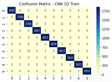
plt.figure(1)
plt.title('Confusion Matrix - CNN 1D Train')
sns.heatmap(ConfusionMatrix(Classification_1D, X_1D_train, y_1D_train) , annot=True, fmt='d',annot_kws={"fontsize":8},cmap="YlGnBu")
plt.show()plt.figure(2)
plt.title('Confusion Matrix - CNN 1D Test')
sns.heatmap(ConfusionMatrix(Classification_1D, X_1D_test, y_1D_test) , annot=True, fmt='d',annot_kws={"fontsize":8},cmap="YlGnBu")
plt.show()plt.figure(3)
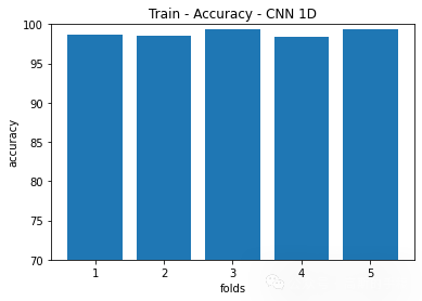
plt.title('Train - Accuracy - CNN 1D')
plt.bar(np.arange(1,kSplits+1),[i*100 for i in accuracy_1D])
plt.ylabel('accuracy')
plt.xlabel('folds')
plt.ylim([70,100])
plt.show()plt.figure(4)
plt.title('Train vs Test Accuracy - CNN 1D')
plt.bar([1,2],[CNN_1D_train_accuracy,CNN_1D_test_accuracy])
plt.ylabel('accuracy')
plt.xlabel('folds')
plt.xticks([1,2],['Train', 'Test'])
plt.ylim([70,100])
plt.show()

二维卷积神经网络2D-CNN分类，不使用时频谱图，直接reshape

Reshape数据

Input_2D = X.reshape([-1,41,41,1])

训练集和测试集划分

X_2D_train, X_2D_test, y_2D_train, y_2D_test = train_test_split(Input_2D, Y_CNN, train_size=0.75,test_size=0.25, random_state=101)

定义2D-CNN分类模型

class CNN_2D():
def __init__(self):
self.model = self.CreateModel()def CreateModel(self):
model = models.Sequential([
layers.Conv2D(filters=16, kernel_size=(3,3), strides=(2,2), padding ='same',activation='relu'),
layers.MaxPool2D(pool_size=(2,2), padding='same'),
layers.Conv2D(filters=32, kernel_size=(3,3),strides=(2,2), padding ='same',activation='relu'),
layers.MaxPool2D(pool_size=(2,2), padding='same'),
layers.Conv2D(filters=64, kernel_size=(3,3),strides=(2,2),padding ='same', activation='relu'),
layers.MaxPool2D(pool_size=(2,2), padding='same'),
layers.Conv2D(filters=128, kernel_size=(3,3),strides=(2,2),padding ='same', activation='relu'),
layers.MaxPool2D(pool_size=(2,2), padding='same'),
layers.Flatten(),
layers.InputLayer(),
layers.Dense(100,activation='relu'),
layers.Dense(50,activation='relu'),
layers.Dense(10),
layers.Softmax()
])
model.compile(optimizer='adam',
loss=tf.keras.losses.CategoricalCrossentropy(),
metrics=['accuracy'])
return modelaccuracy_2D = []

训练模型

for train, test in kfold.split(X_2D_train,y_2D_train):
Classification_2D = CNN_2D()
history = Classification_2D.model.fit(X_2D_train[train], y_2D_train[train], verbose=1, epochs=12)

评估模型在训练集上的准确性

kf_loss, kf_accuracy = Classification_2D.model.evaluate(X_2D_train[test], y_2D_train[test])
accuracy_2D.append(kf_accuracy)CNN_2D_train_accuracy = np.average(accuracy_2D)*100
print('CNN 2D train accuracy =', CNN_2D_train_accuracy)

在测试集上评估模型的准确性

CNN_2D_test_loss, CNN_2D_test_accuracy = Classification_2D.model.evaluate(X_2D_test, y_2D_test)
CNN_2D_test_accuracy*=100
print('CNN 2D test accuracy =', CNN_2D_test_accuracy)

CNN 2D test accuracy = 95.79831957817078

绘制结果

plt.figure(5)
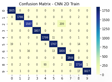
plt.title('Confusion Matrix - CNN 2D Train')
sns.heatmap(ConfusionMatrix(Classification_2D, X_2D_train, y_2D_train) , annot=True, fmt='d',annot_kws={"fontsize":8},cmap="YlGnBu")
plt.show()plt.figure(6)
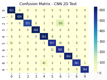
plt.title('Confusion Matrix - CNN 2D Test')
sns.heatmap(ConfusionMatrix(Classification_2D, X_2D_test, y_2D_test) , annot=True, fmt='d',annot_kws={"fontsize":8},cmap="YlGnBu")
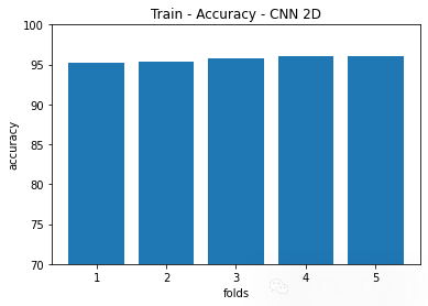
plt.show()plt.figure(7)
plt.title('Train - Accuracy - CNN 2D')
plt.bar(np.arange(1,kSplits+1),[i*100 for i in accuracy_2D])
plt.ylabel('accuracy')
plt.xlabel('folds')
plt.ylim([70,100])
plt.show()plt.figure(8)
plt.title('Train vs Test Accuracy - CNN 2D')
plt.bar([1,2],[CNN_2D_train_accuracy,CNN_2D_test_accuracy])
plt.ylabel('accuracy')
plt.xlabel('folds')
plt.xticks([1,2],['Train', 'Test'])
plt.ylim([70,100])
plt.show()

LSTM分类模型

Reshape数据

Input = X.reshape([-1,1681,1])

训练集和测试集划分

X_train, X_test, y_train, y_test = train_test_split(Input, Y_CNN, train_size=0.75,test_size=0.25, random_state=101)

定义LSTM分类模型

class LSTM_Model():
def __init__(self):
self.model = self.CreateModel()def CreateModel(self):
model = models.Sequential([
layers.LSTM(32, return_sequences=True),
layers.Flatten(),
layers.Dense(10),
layers.Softmax()
])
model.compile(optimizer='adam',
loss=tf.keras.losses.CategoricalCrossentropy(),
metrics=['accuracy'])
return modelaccuracy = []

训练模型

for train, test in kfold.split(X_train,y_train):
Classification = LSTM_Model()
history = Classification.model.fit(X_train[train], y_train[train], verbose=1, epochs=10, use_multiprocessing=True)

评估模型在训练集上的准确性

kf_loss, kf_accuracy = Classification.model.evaluate(X_train[test], y_train[test])
accuracy.append(kf_accuracy)
LSTM_train_accuracy = np.average(accuracy)*100
print('LSTM train accuracy =', LSTM_train_accuracy)

在测试集上评估模型的准确性

LSTM_test_loss, LSTM_test_accuracy = Classification.model.evaluate(X_test, y_test)
LSTM_test_accuracy*=100
print('LSTM test accuracy =', LSTM_test_accuracy)

绘制结果

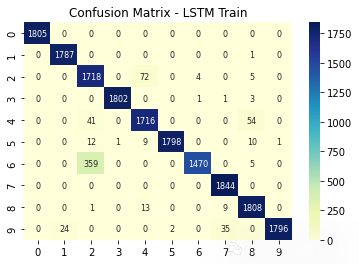
plt.figure(9)
plt.title('Confusion Matrix - LSTM Train')
sns.heatmap(ConfusionMatrix(Classification, X_train, y_train) , annot=True, fmt='d',annot_kws={"fontsize":8},cmap="YlGnBu")
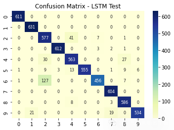
plt.show()plt.figure(10)
plt.title('Confusion Matrix - LSTM Test')
sns.heatmap(ConfusionMatrix(Classification, X_test, y_test) , annot=True, fmt='d',annot_kws={"fontsize":8},cmap="YlGnBu")
plt.show()plt.figure(11)
plt.title('Train - Accuracy - LSTM')
plt.bar(np.arange(1,kSplits+1),[i*100 for i in accuracy])
plt.ylabel('accuracy')
plt.xlabel('folds')
plt.ylim([70,100])
plt.show()plt.figure(12)
plt.title('Train vs Test Accuracy - LSTM')
plt.bar([1,2],[LSTM_train_accuracy,LSTM_test_accuracy])
plt.ylabel('accuracy')
plt.xlabel('folds')
plt.xticks([1,2],['Train', 'Test'])
plt.ylim([70,100])
plt.show()

支持向量机分类模型

输入数据已在 MATLAB 中进行了特征提取，提取的特征为最大值、最小值、峰峰值、均值、方差、标准差、均方根、偏度、波峰因数、时域峰度和幅度等特，共12个

X_Features = scipy.io.loadmat('X_Features.mat')['Feature_Data']
X_Features.shape

(24276, 12)

导入机器学习相关模块

from sklearn.decomposition import PCA
from sklearn.svm import SVC
from sklearn.pipeline import Pipeline
from sklearn.model_selection import GridSearchCV
from sklearn.preprocessing import StandardScaler
from sklearn.decomposition import PCA
from tqdm import tqdm_notebook as tqdm
import warnings
warnings.filterwarnings('ignore')

归一化

X_Norm = StandardScaler().fit_transform(X_Features)

PCA降维，主成分个数取5

pca = PCA(n_components=5)
Input_SVM_np = pca.fit_transform(X_Norm)
Input_SVM = pd.DataFrame(data = Input_SVM_np)
Label_SVM = pd.DataFrame(Y, columns = ['target'])

定义SVM参数

parameters = {'kernel':('rbf','poly','sigmoid'),
'C': [0.01, 1],
'gamma' : [0.01, 1],
'decision_function_shape' : ['ovo']}svm = SVC()

开始训练SVM

训练集测试集划分

X_train_SVM, X_test_SVM, y_train_SVM, y_test_SVM = train_test_split(Input_SVM_np, Y, train_size=0.75,test_size=0.25, random_state=101)

网格搜索参数

svm_cv = GridSearchCV(svm, parameters, cv=5)
svm_cv.fit(X_train_SVM, y_train_SVM)print("Best parameters = ",svm_cv.best_params_)SVM_train_accuracy = svm_cv.best_score_*100
print('SVM train accuracy =', SVM_train_accuracy)

在测试集上评估模型的准确性

SVM_test_accuracy = svm_cv.score(X_test_SVM, y_test_SVM)
SVM_test_accuracy*=100
print('SVM test accuracy =', SVM_test_accuracy)

Best parameters = {'C': 1, 'decision_function_shape': 'ovo', 'gamma': 1, 'kernel': 'rbf'} SVM train accuracy = 92.81046553069329 SVM test accuracy = 92.55231504366452

绘制结果

def ConfusionMatrix_SVM(Model, X, y):
y_pred = Model.predict(X)
ConfusionMat = confusion_matrix(y, y_pred)
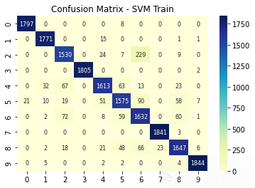
return ConfusionMatprint(svm_cv.score(X_train_SVM, y_train_SVM))plt.figure(13)
plt.title('Confusion Matrix - SVM Train')
sns.heatmap(ConfusionMatrix_SVM(svm_cv, X_train_SVM, y_train_SVM) , annot=True, fmt='d',annot_kws={"fontsize":8},cmap="YlGnBu")
plt.show()plt.figure(14)
plt.title('Confusion Matrix - SVM Test')
sns.heatmap(ConfusionMatrix_SVM(svm_cv, X_test_SVM, y_test_SVM) , annot=True, fmt='d',annot_kws={"fontsize":8},cmap="YlGnBu")
plt.show()plt.figure(16)
plt.title('Train vs Test Accuracy - SVM')
plt.bar([1,2],[SVM_train_accuracy,SVM_test_accuracy])
plt.ylabel('accuracy')
plt.xlabel('folds')
plt.xticks([1,2],['Train', 'Test'])
plt.ylim([70,100])
plt.show()

看一下SVM决策边界

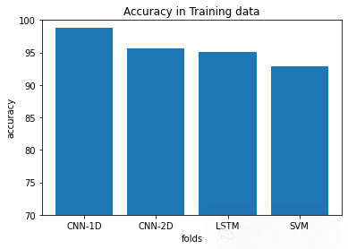
最终的模型性能比较

plt.figure(18)
plt.title('Accuracy in Training data')
plt.bar([1,2,3,4],[CNN_1D_train_accuracy, CNN_2D_train_accuracy, LSTM_train_accuracy, SVM_train_accuracy])
plt.ylabel('accuracy')
plt.xlabel('folds')
plt.xticks([1,2,3,4],['CNN-1D', 'CNN-2D' , 'LSTM', 'SVM'])
plt.ylim([70,100])
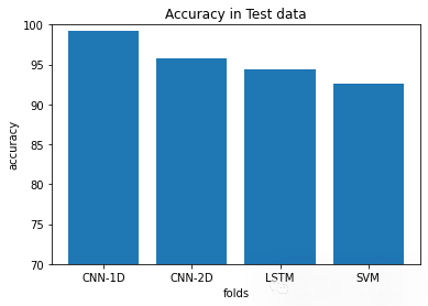
plt.show()plt.figure(19)
plt.title('Accuracy in Test data')
plt.bar([1,2,3,4],[CNN_1D_test_accuracy, CNN_2D_test_accuracy, LSTM_test_accuracy, SVM_test_accuracy])
plt.ylabel('accuracy')
plt.xlabel('folds')
plt.xticks([1,2,3,4],['CNN-1D', 'CNN-2D' , 'LSTM', 'SVM'])
plt.ylim([70,100])
plt.show()