机器学习专项课程03：Unsupervised Learning, Recommenders, Reinforcement Learning笔记 Week02

本文主要是介绍机器学习专项课程03：Unsupervised Learning, Recommenders, Reinforcement Learning笔记 Week02，希望对大家解决编程问题提供一定的参考价值，需要的开发者们随着小编来一起学习吧！

Week 02 of Unsupervised Learning, Recommenders, Reinforcement Learning

课程地址： https://www.coursera.org/learn/unsupervised-learning-recommenders-reinforcement-learning

本笔记包含字幕，quiz的答案以及作业的代码，仅供个人学习使用，如有侵权，请联系删除。

Learning Objectives

---

• Implement collaborative filtering recommender systems in TensorFlow
• Implement deep learning content based filtering using a neural network in TensorFlow
• Understand ethical considerations in building recommender systems

[1] Collaborative filtering

Making recommendations

Welcome to this second to last week of
the machine learning specialization. I’m really happy that together,
almost all the way to the finish line. What we’ll do this week is
discuss recommended systems. This is one of the topics that has
received quite a bit of attention in academia. But the commercial impact and the actual number of practical use cases
of recommended systems seems to me to be even vastly greater than the amount of
attention it has received in academia.

Every time you go to an online
shopping website like Amazon or a movie streaming sites like Netflix or
go to one of the apps or sites that do food delivery. Many of these sites will recommend things
to you that they think you may want to buy or movies they think you
may want to watch or restaurants that they think
you may want to try out.

And for many companies, a large fraction of sales is driven
by their recommended systems. So today for many companies, the economics
or the value driven by recommended systems is very large and so what we’re doing this
week is take a look at how they work. So with that let’s dive in and take
a look at what is a recommended system.

预测电影排名的例子

I’m going to use as a running example, the
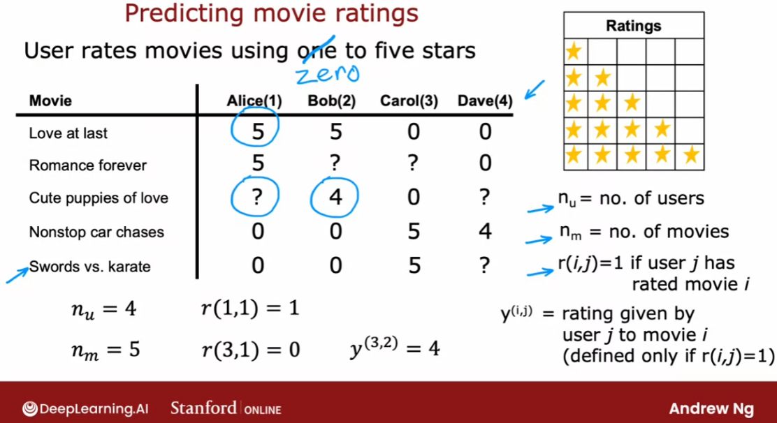
application of predicting movie ratings. So say you run a large
movie streaming website and your users have rated movies
using one to five stars. And so in a typical recommended
system you have a set of users, here we have four users Alice,
Bob Carol and Dave. Which have numbered users 1,2,3,4. As well as a set of movies Love at last,
Romance forever, Cute puppies of love and then Nonstop
car chases and Sword versus karate. And what the users have done is rated
these movies one to five stars. Or in fact to make some of these
examples a little bit easier. I’m not going to let them rate
the movies from zero to five stars.

So say Alice has rated Love and last
five stars, Romance forever five stars. Maybe she has not yet
watched cute puppies of love so you don’t have a rating for that. And I’m going to denote that
via a question mark and she thinks nonstop car chases and sword
versus karate deserve zero stars bob. Race at five stars has not watched that,
so you don’t have a rating
race at four stars, 0,0.

Carol on the other hand,
thinks that deserve zero stars has not watched that zero stars and
she loves nonstop car chases and swords versus karate and
Dave rates the movies as follows. In the typical recommended system, you have some number of users
as well as some number of items. In this case the items are movies that
you want to recommend to the users. And even though I’m using movies in this
example, the same logic or the same thing works for recommending anything from
products or websites to my self, to restaurants, to even which media articles,
the social media articles to show, to the user that may be
more interesting for them.

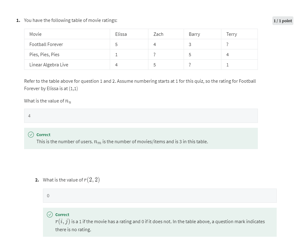
The notation I’m going to use is I’m going
to use nu to denote the number of users. So in this example nu is equal to
four because you have four users and nm to denote the number of movies or
really the number of items. So in this example nm is equal to
five because we have five movies.

I’m going to set r(i,j)=1, if user j has rated movie i. So for example, use a one
Dallas Alice has rated movie one but has not rated movie three and
so r(1,1) =1, because she has rated movie one, but r( 3,1)=0 because she has not
rated movie number three.

Then finally I’m going to use y(i,j). J to denote the rating
given by user j to movie i. So for example, this rating here would be that movie three
was rated by user 2 to be equal to four. Notice that not every user rates
every movie and it’s important for the system to know which users
have rated which movies. That’s why we’re going to define
r(i,j)=1 if user j has rated movie i and will be equal to zero if user
j has not rated movie i.

So with this framework for recommended
systems one possible way to approach the problem is to look at the movies
that users have not rated. And to try to predict how users would
rate those movies because then we can try to recommend to users things that they
are more likely to rate as five stars.

And in the next video we’ll start
to develop an algorithm for doing exactly that. But making one very special assumption. Which is we’re going to assume temporarily
that we have access to features or extra information about the movies such
as which movies are romance movies, which movies are action movies. And using that will start
to develop an algorithm. But later this week will actually come
back and ask what if we don’t have these features, how can you still
get the algorithm to work then? But let’s go on to the next video to
start building up this algorithm.

Using per-item features

So let’s take a look at how we can
develop a recommender system if we had features of each item, or
features of each movie. So here’s the same data set that we
had previously with the four users having rated some but
not all of the five movies.

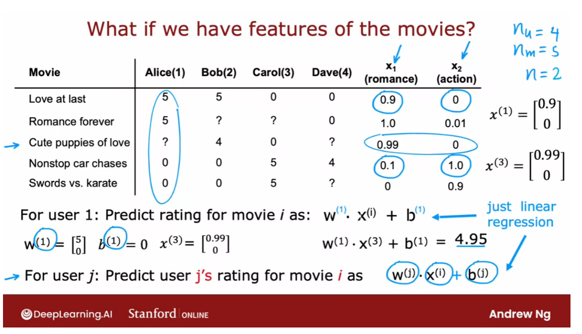
What if we additionally have
features of the movies? So here I’ve added two features X1 and
X2, that tell us how much each of these is a romance movie, and
how much each of these is an action movie. So for example Love at Last
is a very romantic movie, so this feature takes on 0.9, but
it’s not at all an action movie. So this feature takes on 0.

But it turns out Nonstop Car chases has
just a little bit of romance in it. So it’s 0.1, but it has a ton of action. So that feature takes on the value of 1.0. So you recall that I had used the notation
nu to denote the number of users, which is 4 and m to denote
the number of movies which is 5. I’m going to also introduce n to denote
the number of features we have here. And so n=2, because we have two
features X1 and X2 for each movie.

With these features we have for
example that the features for movie one, that is the movie Love at Last,
would be 0.90. And the features for the third movie Cute Puppies of Love would be 0.99 and 0.

And let’s start by taking a look at
how we might make predictions for Alice’s movie ratings. So for user one, that is Alice, let’s say we predict the rating for movie i as w.X(i)+b. So this is just a lot
like linear regression. For example if we end up choosing
the parameter w(1)=[5,0] and say b(1)=0, then the prediction for movie three where
the features are 0.99 and 0, which is just copied from here,
first feature 0.99, second feature 0. Our prediction would be w.X(3)+b=0.99 times 5 plus 0 times zero, which turns out to be equal to 4.95.

And this rating seems pretty plausible. It looks like Alice has given high ratings
to Love at Last and Romance Forever, to two highly romantic movies, but
given low ratings to the action movies, Nonstop Car Chases and Swords vs Karate. So if we look at Cute Puppies of Love, well predicting that she might rate
that 4.95 seems quite plausible. And so these parameters w and b for Alice seems like a reasonable model for
predicting her movie ratings.

Just add a little the notation
because we have not just one user but multiple users, or
really nu equals 4 users. I’m going to add a superscript 1 here to
denote that this is the parameter w(1) for user 1 and
add a superscript 1 there as well. And similarly here and here as well,
so that we would actually have different parameters for
each of the 4 users on data set.

And more generally in this
model we can for user j, not just user 1 now,
we can predict user j’s rating for movie i as w(j).X(i)+b(j). So here the parameters w(j) and b(j) are the parameters used
to predict user j’s rating for movie i which is a function of X(i),
which is the features of movie i. And this is a lot like linear regression,
except that we’re fitting a different linear regression model for
each of the 4 users in the dataset.

So let’s take a look at how we can
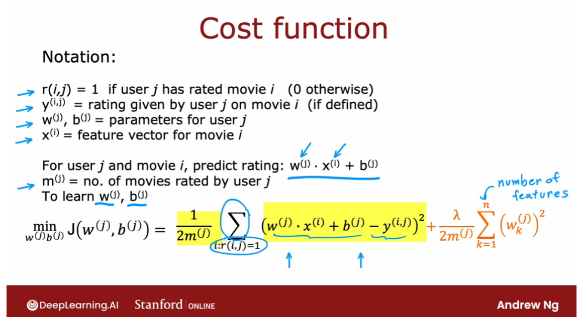
formulate the cost function for this algorithm. As a reminder, our notation
is that r(i.,j)=1 if user j has rated movie i or
0 otherwise. And y(i,j)=rating given
by user j on movie i. And on the previous side we defined w(j),
b(j) as the parameters for user j. And X(i) as the feature vector for
movie i. So the model we have is for user j and movie i predict the rating
to be w(j).X(i)+b(j).

I’m going to introduce just
one new piece of notation, which is I’m going to use m(j) to denote
the number of movies rated by user j. So if the user has rated 4 movies,
then m(j) would be equal to 4. And if the user has rated 3 movies
then m(j) would be equal to 3. So what we’d like to do is to
learn the parameters w(j) and b(j), given the data that we have. That is given the ratings a user
has given of a set of movies. So the algorithm we’re going to use is
very similar to linear regression.

Cost function 很像线性回归

So let’s write out the cost function for
learning the parameters w(j) and b(j) for a given user j. And let’s just focus on one
user on user j for now. I’m going to use the mean
squared error criteria. So the cost will be the prediction,
which is w(j).X(i)+b(j) minus the actual rating
that the user had given. So minus y(i,j) squared. And we’re trying to
choose parameters w and b to minimize the squared error
between the predicted rating and the actual rating that was observed. But the user hasn’t rated all the movies,
so if we’re going to sum over this,
we’re going to sum over only over the values
of i where r(i,j)=1. So we’re going to sum only over the movies
i that user j has actually rated.

So that’s what this denotes,
sum of all values of i where r(i,j)=1. Meaning that user j has
rated that movie i. And then finally we can take
the usual normalization 1 over m(j). And this is very much like
the cost function we have for linear regression with m or
really m(j) training examples. Where you’re summing over the m(j) movies
for which you have a rating taking a squared error and
the normalizing by this 1 over 2m(j).

And this is going to be a cost function J of w(j), b(j). And if we minimize this as
a function of w(j) and b(j), then you should come up with a pretty
good choice of parameters w(i) and b(j). For making predictions for
user j’s ratings. Let me have just one more
term to this cost function, which is the regularization
term to prevent overfitting. And so
here’s our usual regularization parameter, lambda divided by 2m(j) and then times as sum of the squared
values of the parameters w. And so
n is a number of numbers in X(i) and that’s the same as a number
of numbers in w(j).

If you were to minimize this cost
function J as a function of w and b, you should get a pretty
good set of parameters for predicting user j’s ratings for
other movies. Now, before moving on, it turns out
that for recommender systems it would be convenient to actually eliminate
this division by m(j) term, m(j) is just a constant
in this expression. And so, even if you take it out, you should end up with
the same value of w and b.

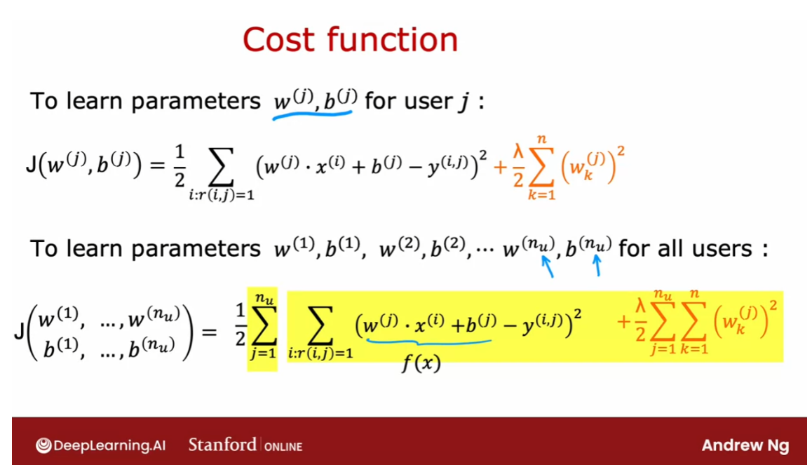
Now let me take this cost function
down here to the bottom and copy it to the next slide. So we have that to learn
the parameters w(j), b(j) for user j. We would minimize this cost function
as a function of w(j) and b(j). But instead of focusing on a single user, let’s look at how we learn
the parameters for all of the users. To learn the parameters w(1), b(1), w(2), b(2),…,w(nu), b(nu), we would take this cost function on
top and sum it over all the nu users. So we would have sum from
j=1 one to nu of the same cost function that we
had written up above. And this becomes the cost for learning all the parameters for
all of the users.

And if we use gradient descent or any other optimization algorithm to
minimize this as a function of w(1), b(1) all the way through w(nu),
b(nu), then you have a pretty good set of parameters for predicting
movie ratings for all the users. And you may notice that this algorithm
is a lot like linear regression, where that plays a role similar to
the output f(x) of linear regression.

Only now we’re training a different linear
regression model for each of the nu users. So that’s how you can learn parameters and
predict movie ratings, if you had access to these features X1 and
X2. That tell you how much is each of
the movies, a romance movie, and how much is each of
the movies an action movie?

But where do these features come from? And what if you don’t have access to such
features that give you enough detail about the movies with which
to make these predictions? In the next video, we’ll look at
the modification of this algorithm. They’ll let you make predictions
that you make recommendations. Even if you don’t have, in advance,
features that describe the items of the movies in sufficient detail to
run the algorithm that we just saw. Let’s go on and
take a look at that in the next video

Collaborative filtering algorithm

In the last video, you saw how if you have features
for each movie, such as features x_1 and x_2
that tell you how much is this a romance movie and how much is this an action movie. Then you can use basically
linear regression to learn to predict
movie ratings. But what if you don’t have
those features, x_1 and x_2?

Let’s take a look at how
you can learn or come up with those features x_1
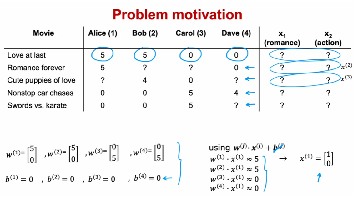
and x_2 from the data. Here’s the data
that we had before. But what if instead of having these numbers
for x_1 and x_2, we didn’t know in advance what the values of the features
x_1 and x_2 were? I’m going to replace them with
question marks over here. Now, just for the
purposes of illustration, let’s say we had somehow already learned parameters
for the four users. Let’s say that we
learned parameters w^1 equals 5 and 0 and b^1
equals 0, for user one. W^2 is also 5, 0 b^2, 0. W^3 is 0, 5 b^3 is 0, and for user four W^4 is also 0, 5 and b^4 0, 0.

We’ll worry later about
how we might have come up with these
parameters, w and b. But let’s say we
have them already. As a reminder, to predict
user j’s rating on movie i, we’re going to use
w^j dot product, the features of x_i plus b^j. To simplify this example, all the values of b are
actually equal to 0. Just to reduce a
little bit of writing, I’m going to ignore b for
the rest of this example.

Let’s take a look at
how we can try to guess what might be reasonable
features for movie one. If these are the parameters
you have on the left, then given that Alice
rated movie one, 5, we should have that w^1.x1
should be about equal to 5 and w^2.x2 should also be about equal to 5
because Bob rated it 5. W^3.x1 should be close to 0 and w^4.x1 should be
close to 0 as well.

The question is, given these values for w
that we have up here, what choice for x_1 will cause
these values to be right? Well, one possible
choice would be if the features for
that first movie, were 1, 0 in which case, w^1.x1 will be equal to 5, w^2.x1 will be equal
to 5 and similarly, w^3 or w^4 dot product with this feature vector x_1
would be equal to 0. What we have is that if you have the parameters for
all four users here, and if you have four ratings in this example that you
want to try to match, you can take a reasonable
guess at what lists a feature vector x_1 for movie one that would make good predictions for these four
ratings up on top.

Similarly, if you have
these parameter vectors, you can also try to come up with a feature vector x_2
for the second movie, feature vector x_3
for the third movie, and so on to try to make the
algorithm’s predictions on these additional movies close to what was actually the
ratings given by the users.

Let’s come up with a cost
function for actually learning the values
of x_1 and x_2. By the way, notice
that this works only because we have parameters
for four users. That’s what allows us to try to guess appropriate
features, x_1. This is why in a typical
linear regression application if you had just a single user, you don’t actually have enough information to figure out what would be the features, x_1 and x_2, which is why in the linear regression contexts
that you saw in course 1, you can’t come up with features
x_1 and x_2 from scratch.

But in collaborative filtering, is because you have ratings from multiple users of the same
item with the same movie. That’s what makes it
possible to try to guess what are possible
values for these features.

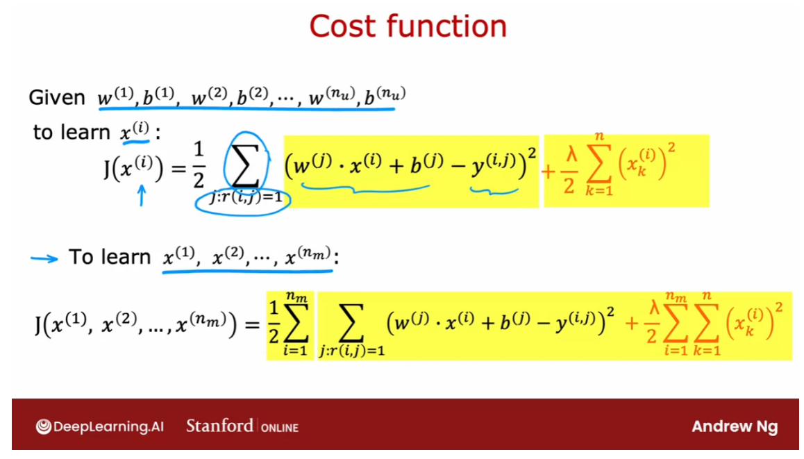
Given w^1, b^1, w^2, b^2, and so on through
w^n_u and b^n_u, for the n subscript u users. If you want to learn the features x^i for
a specific movie, i is a cost function we
could use which is that. I’m going to want to minimize
squared error as usual. If the predicted rating by user j on movie i
is given by this, let’s take the
squared difference from the actual
movie rating y,i,j.

As before, let’s sum
over all the users j. But this will be a sum over all values of j, where r, i, j is equal to I. I’ll add
a 1.5 there as usual. As I defined this as a
cost function for x^i. Then if we minimize this
as a function of x^i you be choosing the
features for movie i. So therefore all the users
J that have rated movie i, we will try to minimize the
squared difference between what your choice of features
x^i results in terms of the predicted movie rating minus the actual movie rating
that the user had given it. Then finally, if we want to
add a regularization term, we add the usual
plus Lambda over 2, K equals 1 through n, where n as usual
is the number of features of x^i squared.

Lastly, to learn
all the features x1 through x^n_m because
we have n_m movies, we can take this
cost function on top and sum it over
all the movies. Sum from i equals 1 through the number of movies
and then just take this term from above
and this becomes a cost function for learning the features for all of
the movies in the dataset. So if you have parameters
w and b, all the users, then minimizing this cost
function as a function of x1 through x^n_m using gradient descent
or some other algorithm, this will actually allow you
to take a pretty good guess at learning good
features for the movies.

This is pretty remarkable for most machine
learning applications the features had to be externally given but
in this algorithm, we can actually learn the
features for a given movie.

But what we’ve done
so far in this video, we assumed you had those parameters w and b
for the different users. Where do you get those
parameters from? Well, let’s put together
the algorithm from the last video for learning
w and b and what we just talked about in this
video for learning x and that will give us our
collaborative filtering algorithm.

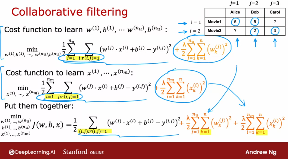
Here’s the cost function
for learning the features. This is what we had
derived on the last slide. Now, it turns out that if
we put these two together, this term here is exactly
the same as this term here. Notice that sum over
j of all values of i is that r,i,j
equals 1 is the same as summing
over all values of i with all j where
r,i,j is equal to 1. This summation is
just summing over all user movie pairs
where there is a rating.

What I’m going to do is put these two cost functions
together and have this where I’m just writing
out the summation more explicitly as summing
over all pairs i and j, where we do have a rating of the usual squared cost
function and then let me take the regularization term from learning the
parameters w and b, and put that here and take the regularization term from learning the features
x and put them here and this ends up being our overall cost function
for learning w, b, and x.

It turns out that
if you minimize this cost function as a
function of w and b as well as x, then this algorithm
actually works. Here’s what I mean. If
we had three users and two movies and if you have
ratings for these four movies, but not those two,
over here does, is it sums over all the users. For user 1 has determined
the cost function for this, for user 2 has determined
the cost function for this, for user 3 has determined
the cost function for this. We’re summing over
users first and then having one term for each movie where
there is a rating.

But an alternative way to
carry out the summation is to first look at movie 1, that’s what this
summation here does, and then to include all the
users that rated movie 1, and then look at movie
2 and have a term for all the users that
had rated movie 2. You see that in both cases
we’re just summing over these four areas where the user had rated the
corresponding movie. That’s why this summation on top and this
summation here are the two ways of summing over all of the pairs where the
user had rated that movie.

介绍协同过滤算法

协同过滤算法是一种推荐系统算法，它基于用户之间的相似性或物品之间的相似性来进行推荐。这种算法主要分为两种类型：基于用户的协同过滤和基于物品的协同过滤。

1. 基于用户的协同过滤（User-Based Collaborative Filtering）：

   • 这种方法首先找出与目标用户相似兴趣或行为的其他用户集合，然后利用这些相似用户的历史行为来预测目标用户可能喜欢的物品。
   • 该方法的步骤包括计算用户之间的相似性（通常使用相关系数或余弦相似度等度量），然后利用这些相似性权重对相似用户的评分进行加权平均，从而预测目标用户对尚未评价的物品的评分或偏好。

2. 基于物品的协同过滤（Item-Based Collaborative Filtering）：

   • 这种方法首先计算物品之间的相似性，然后根据目标用户已经喜欢的物品找出相似的物品，进而进行推荐。
   • 相似性的计算通常使用物品之间的共同被喜欢程度或其他相似性指标。一旦计算出物品之间的相似性，就可以向用户推荐那些与其已经喜欢的物品相似的物品。

协同过滤算法的优点是它能够提供个性化的推荐，而无需事先对物品进行明确的特征提取或建模。但是，它也有一些缺点，例如冷启动问题（对于新用户或新物品如何进行推荐）、数据稀疏性（用户-物品评分矩阵往往非常稀疏）、可扩展性（随着用户和物品数量的增加，计算复杂度会增加）等。

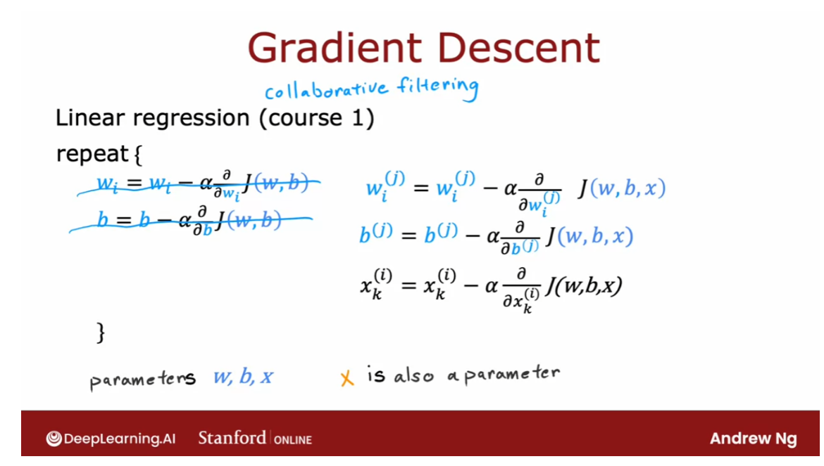
How do you minimize
this cost function as a function of w, b, and x? One thing you could do is
to use gradient descent. In course 1 when we learned
about linear regression, this is the gradient descent
algorithm you had seen, where we had the
cost function J, which is a function of
the parameters w and b, and we’d apply gradient
descent as follows.

With collaborative filtering,
the cost function is in a function of just w and
b is now a function of w, b, and x. I’m using w and b here to denote
the parameters for all of the users and x here just informally to denote the
features of all of the movies. But if you’re able to take partial derivatives with respect to the different parameters, you can then continue to update the parameters as follows.

But now we need to optimize this with respect to x as well. We also will want
to update each of these parameters x using
gradient descent as follows. It turns out that
if you do this, then you actually find
pretty good values of w and b as well as x. In this formulation
of the problem, the parameters of w and b, and x is also a parameter. Then finally, to learn
the values of x, we also will update x as x minus the partial derivative
respect to x of the cost w, b, x.

I’m using the
notation here a little bit informally and not keeping very careful track of the
superscripts and subscripts, but the key takeaway I
hope you have from this is that the parameters to
this model are w and b, and x now is also a parameter, which is why we minimize
the cost function as a function of all three of
these sets of parameters, w and b, as well as x.

The algorithm we derived is called collaborative filtering, and the name
collaborative filtering refers to the sense that because multiple users have rated the same movie
collaboratively, given you a sense of what
this movie maybe like, that allows you to guess what are appropriate features
for that movie, and this in turn allows you to predict how other users that haven’t yet rated
that same movie may decide to rate
it in the future. This collaborative filtering is this gathering of data
from multiple users. This collaboration between
users to help you predict ratings for even other
users in the future.

协同过滤算法是一种基于多个用户共同对同一部电影（或物品）进行评价的数据，来推断用户对未来尚未评价的电影可能的评价的算法。通过多个用户的合作，共同提供了对电影的评价数据，这些数据被用来猜测该电影的特征，进而预测其他用户对该电影的评价。协同过滤算法依赖于多个用户之间的合作和数据共享，以帮助预测其他用户未来的评价。

So far, our problem
formulation has used movie ratings from 1- 5
stars or from 0- 5 stars. A very common use case of
recommender systems is when you have binary labels such
as that the user favors, or like, or interact
with an item. In the next video, let’s take
a look at a generalization of the model that you’ve seen
so far to binary labels. Let’s go see that
in the next video.

Binary labels: favs, likes and clicks

Many important applications
of recommender systems or collective filtering algorithms
involved binary labels where instead of a user giving you a one to five star or
zero to five star rating, they just somehow give you a sense of they like
this item or they did not like this item.

Let’s take a look at how to generalize
the algorithm you’ve seen to this setting. The process we’ll use to generalize the
algorithm will be very much reminiscent to how we have gone from linear regression
to logistic regression, to predicting numbers to predicting a binary label
back in course one, let’s take a look.

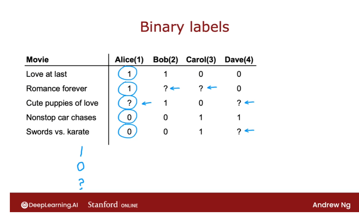
Here’s an example of a collaborative
filtering data set with binary labels. A one the notes that the user liked or
engaged with a particular movie. So label one could mean that Alice watched
the movie Love at last all the way to the end and watch romance
forever all the way to the end. But after playing a few minutes of nonstop
car chases decided to stop the video and move on. Or it could mean that she
explicitly hit like or favorite on an app to indicate
that she liked these movies. But after checking out
nonstop car chasers and swords versus karate did not hit like. And the question mark usually means
the user has not yet seen the item and so they weren’t in a position to decide
whether or not to hit like or favorite on that particular item.

So the question is how can we take the
collaborative filtering algorithm that you saw in the last video and
get it to work on this dataset. And by predicting how likely Alice,
Bob carol and Dave are to like the items
that they have not yet rated, we can then decide how much we should
recommend these items to them. There are many ways of defining what is
the label one and what is the label zero, and what is the label question mark in
collaborative filtering with binary labels.

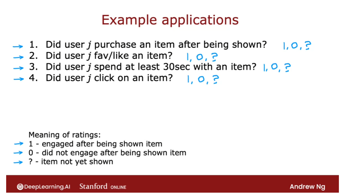
Let’s take a look at a few examples. In an online shopping website,
the label could denote whether or not user j chose to purchase
an item after they were exposed to it, after they were shown the item. So one would denote that they purchase
it zero would denote that they did not purchase it. And the question mark would denote that
they were not even shown were not even exposed to the item.

Or in a social media setting,
the labels one or zero could denote did the user favorite or
like an item after they were shown it. And question mark would be if they
have not yet been shown the item

or many sites instead of asking for
explicit user rating will use the user behavior to try to
guess if the user like the item. So for example, you can measure if a user
spends at least 30 seconds of an item. And if they did, then assign that a label
one because the user found the item engaging or
if a user was shown an item but did not spend at least 30 seconds with it,
then assign that a label zero. Or if the user was not shown the item yet,
then assign it a question mark.

Another way to generate a rating
implicitly as a function of the user behavior will be to see
that the user click on an item. This is often done in online advertising
where if the user has been shown an ad, if they clicked on it
assign it the label one, if they did not click assign it the
label zero and the question mark were referred to if the user has not even
been shown that ad in the first place.

So often these binary labels will
have a rough meaning as follows. A label of one means that the user
engaged after being shown an item And engaged could mean that they clicked or
spend 30 seconds or explicitly favorite or
like to purchase the item.

A zero will reflect the user not
engaging after being shown the item, the question mark will reflect the item
not yet having been shown to the user.

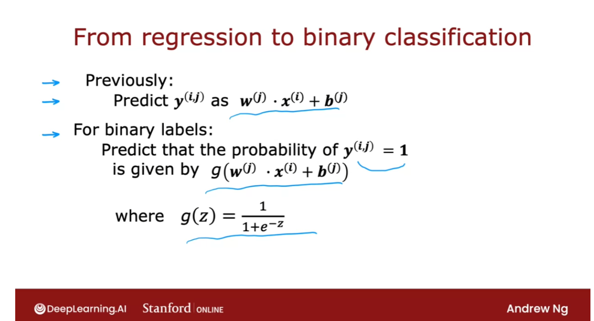
So given these binary labels, let’s look at how we can generalize our
algorithm which is a lot like linear regression from the previous couple videos
to predicting these binary outputs. Previously we were predicting
label yij as wj.xi+b. So this was a lot like
a linear regression model.

For binary labels, we’re going to predict that the probability of yijb=1
is given by not wj.xi+b. But it said by g of this formula, where now g(z) 1/(1 +e to the -z). So this is the logistic function just
like we saw in logistic regression. And what we would do is take what was
a lot like a linear regression model and turn it into something that would
be a lot like a logistic regression model where will now predict
the probability of yij being 1 that is of the user having engaged
with or like the item using this model.

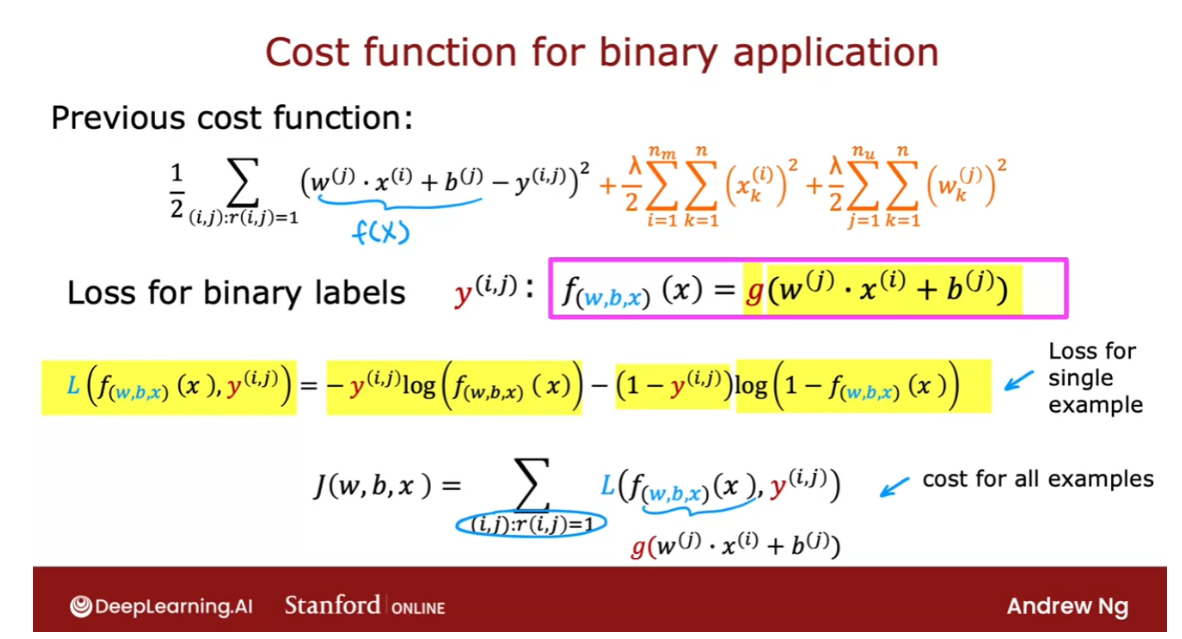
In order to build this algorithm, we’ll also have to modify the cost
function from the squared error cost function to the cost function
that is more appropriate for binary labels for
a logistic regression like model. So previously, this was the cost
function that we had where this term play their role similar to f(x),
the prediction of the algorithm. When you now have binary labels, yij when the labels are one or zero or question mark, then the prediction f(x) becomes instead of wj.xi+b j it becomes g of this where g is the logistic function.

And similar to when we had
derived logistic regression, we had written out
the following loss function for a single example which was at the loss
if the algorithm predicts f(x) and the true label was y, the loss was this. It was -y log f-y log 1-f. This is also sometimes called
the binary cross entropy cost function.

But this is a standard cost function that
we used for logistic regression as was for the binary classification problems
when we’re training neural networks. And so to adapt this to
the collaborative filtering setting, let me write out the cost function
which is now a function of all the parameters w and
b as well as all the parameters x which are the features of
the individual movies or items of. We now need to sum over all
the pairs ij where riij=1 notice this is just similar to
the summation up on top.

And now instead of this
squared error cost function, we’re going to use that loss function. There’s a function of f(x), yij. Where f(x) here? That’s my abbreviation. My shorthand for g(wj.x1+bj). As we plug this into here,
then this gives you the cost function they could use for
collaborative filtering on binary labels.

So that’s it. That’s how you can take
the linear regression, like collaborative filtering algorithm and
generalize it to work with binary labels. And this actually very significantly opens
up the set of applications you can address with this algorithm.

Now, even though you’ve
seen the key structure and cost function of the algorithm,
there are also some implementation, all tips that will make your
algorithm work much better. Let’s go on to the next video to take a
look at some details of how you implement it and some little modifications
that make the algorithm run much faster. Let’s go on to the next video.

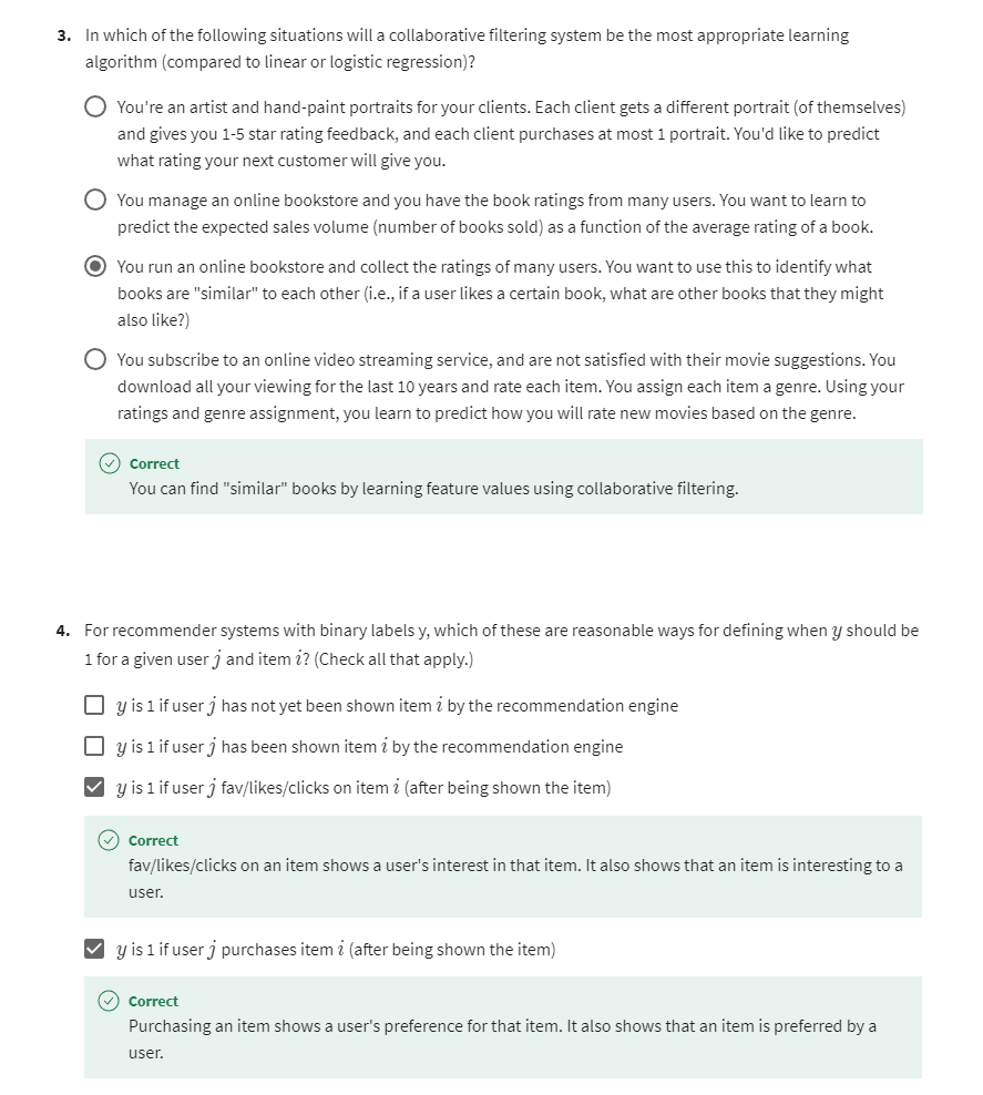
[2] Practice quiz: Collaborative filtering

第三题第一次尝试做错

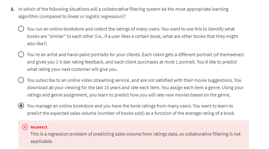
第三题第二次尝试

[3] Recommender systems implementation detail

Mean normalization

Back in the first course,
you have seen how for linear regression, future normalization can help
the algorithm run faster. In the case of building
a recommended system with numbers wide such as movie
ratings from one to five or zero to five stars, it turns out your
algorithm will run more efficiently. And also perform a bit better if you
first carry out mean normalization.

That is if you normalize the movie ratings
to have a consistent average value, let’s take a look at what that means. So here’s the data set
that we’ve been using. And down below is the cost function
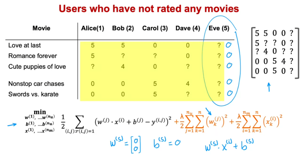
you used to learn the parameters for the model. In order to explain mean normalization, I’m going to add fifth user
Eve who has not yet rated any movies. And you see in a little bit that
adding mean normalization will help the algorithm make better
predictions on the user Eve.

In fact, if you were to train
a collaborative filtering algorithm on this data, then because we
are trying to make the parameters w small because of this regularization term. If you were to run
the algorithm on this dataset, you actually end up with
the parameters w for the fifth user, for the user Eve to be equal to [0
0] as well as quite likely b(5) = 0. Because Eve hasn’t rated any movies yet,
the parameters w and b don’t affect this first term in
the cost function because none of Eve’s movie’s rating play a role in
this squared error cost function.

And so minimizing this means making
the parameters w as small as possible. We didn’t really regularize b. But if you initialize b to 0 as the
default, you end up with b(5) = 0 as well. But if these are the parameters for
user 5 that is for Eve, then what the average
will end up doing is predict that all of Eve’s movies ratings
would be w(5) dot x for movie i + b(5). And this is equal to 0 if w and
b above equals 0. And so this algorithm will predict that
if you have a new user that has not yet rated anything, we think they’ll
rate all movies with zero stars and that’s not particularly helpful.

So in this video, we’ll see that
mean normalization will help this algorithm come up with better
predictions of the movie ratings for a new user that has not yet
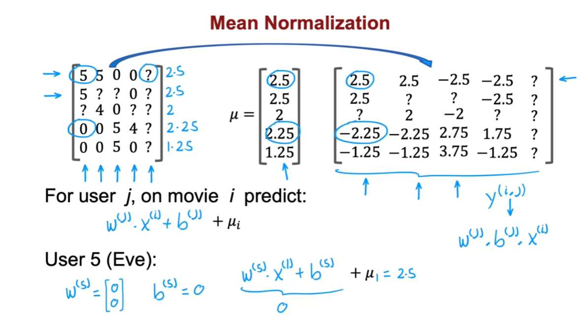
rated any movies. In order to describe mean normalization, let me take all of the values here
including all the question marks for Eve and put them in a two
dimensional matrix like this. Just to write out all the ratings
including the question marks in a more sustained and more compact way.

To carry out mean normalization, what we’re going to do is take
all of these ratings and for each movie,
compute the average rating that was given. So movie one had two 5s and two 0s and
so the average rating is 2.5. Movie two had a 5 and a 0,
so that averages out to 2.5. Movie three 4 and 0 averages out to 2. Movie four averages out to 2.25 rating. And movie five not that popular,
has an average 1.25 rating. So I’m going to take all
of these five numbers and gather them into a vector which I’m
going to call μ because this is the vector of the average ratings that
each of the movies had.

Averaging over just the users that
did read that particular movie. Instead of using these original 0
to 5 star ratings over here, I’m going to take this and subtract from every
rating the mean rating that it was given. So for example this movie rating was 5. I’m going to subtract 2.5
giving me 2.5 over here. This movie had a 0 star rating. I’m going to subtract 2.25 giving
me a -2.25 rating and so on for all of the now five users including the new
user Eve as well as for all five movies.

Then these new values on the right
become your new values of Y(i,j). We’re going to pretend that user 1 had
given a 2.5 rating to movie one and the -2.25 rating to movie four. And using this, you can then learn w(j), b(j) and x(i) same as before for
user j on movie i, you would predict w(j).x(i) + b(j). But because we had subtracted off µi for
movie i during this mean normalization step,
in order to predict not a negative star rating which is impossible for
user rates from 0 to 5 stars. We have to add back this µi which is
just the value we have subtracted out.

So as a concrete example,
if we look at what happens with user 5 with the new user Eve because
she had not yet rated any movies, the average might learn parameters
w(5) = [0 0] and say b(5) = 0. And so
if we look at the predicted rating for movie one, we will predict that Eve will rate it w(5).x1 + b(5) but this is 0 and then + µ1 which is equal to 2.5. So this seems more reasonable to think
Eve is likely to rate this movie 2.5 rather than think Eve will rate
all movie zero stars just because she hasn’t rated any movies yet.

And in fact the effect of this
algorithm is it will cause the initial guesses for
the new user Eve to be just equal to the mean of whatever other users
have rated these five movies. And that seems more reasonable to
take the average rating of the movies rather than to guess that all
the ratings by Eve will be zero. It turns out that by normalizing
the mean of the different movies ratings to be zero, the optimization algorithm for the recommender system will also
run just a little bit faster.

But it does make the algorithm
behave much better for users who have rated no movies or
very small numbers of movies. And the predictions will
become more reasonable. In this example, what we did was normalize each of the rows
of this matrix to have zero mean and we saw this helps when there’s a new user
that hasn’t rated a lot of movies yet.

There’s one other alternative that
you could use which is to instead normalize the columns of this
matrix to have zero mean. And that would be
a reasonable thing to do too. But I think in this application,
normalizing the rows so that you can give reasonable ratings for a new user seems more important
than normalizing the columns.

Normalizing the columns would hope if
there was a brand new movie that no one has rated yet. But if there’s a brand new movie
that no one has rated yet, you probably shouldn’t show that movie
to too many users initially because you don’t know that much about that movie. So normalizing columns the hope with
the case of a movie with no ratings seems less important to me
than normalizing the rules to hope with the case of a new user
that’s hardly rated any movies yet.

And when you are building your own
recommended system in this week’s practice lab, normalizing just
the rows should work fine. So that’s mean normalization. It makes the algorithm
run a little bit faster. But even more important, it makes
the algorithm give much better, much more reasonable predictions when there
are users that rated very few movies or even no movies at all. This implementation detail of mean
normalization will make your recommended system work much better. Next, let’s go into the next video to
talk about how you can implement this for yourself in TensorFlow.

TensorFlow implementation of collaborative filtering

In this video, we’ll take a look at how
you can use TensorFlow to implement the collaborative filtering algorithm. You might be used to thinking
of TensorFlow as a tool for building neural networks. And it is. It’s a great tool for
building neural networks. And it turns out that TensorFlow
can also be very helpful for building other types of
learning algorithms as well. Like the collaborative
filtering algorithm.

One of the reasons I like using TensorFlow
for talks like these is that for many applications in order to
implement gradient descent, you need to find the derivatives of
the cost function, but TensorFlow can automatically figure out for you what
are the derivatives of the cost function.

All you have to do is implement the cost
function and without needing to know any calculus, without needing
to take derivatives yourself, you can get TensorFlow with
just a few lines of code to compute that derivative term, that can
be used to optimize the cost function.

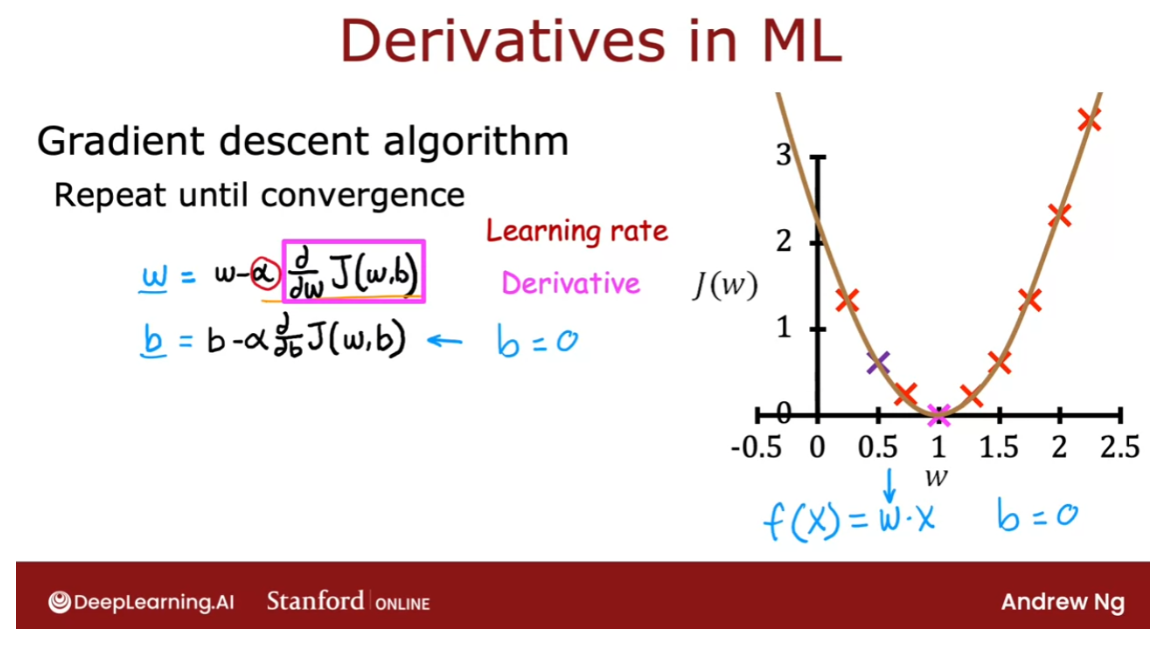
Let’s take a look at how all this works. You might remember this diagram
here on the right from course one. This is exactly the diagram that
we had looked at when we talked about optimizing w. When we were working through our
first linear regression example. And at that time we had set b=0. And so
the model was just predicting f(x)=w.x. And we wanted to find the value of w
that minimizes the cost function J.

So the way we were doing that was
via a gradient descent update, which looked like this,
where w gets repeatedly updated as w minus the learning rate alpha
times the derivative term. If you are updating b as well,
this is the expression you will use. But if you said b=0,
you just forgo the second update and you keep on performing this gradient
descent update until convergence.

Sometimes computing this derivative or
partial derivative term can be difficult. And it turns out that
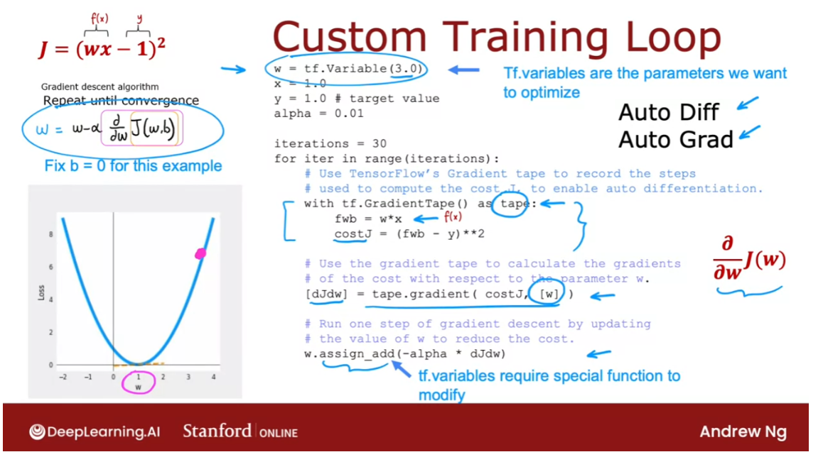
TensorFlow can help with that. Let’s see how. I’m going to use a very simple cost function J=(wx-1) squared. So wx is our simplified f w of x and y is equal to 1. And so this would be the cost
function if we had f(x) equals wx,y equals 1 for
the one training example that we have, and if we were not optimizing
this respect to b. So the gradient descent algorithm
will repeat until convergence this update over here.

It turns out that if you implement
the cost function J over here, TensorFlow can automatically compute for you this derivative term and
thereby get gradient descent to work. I’ll give you a high level overview of
what this code does, w=tf.variable(3.0). Takes the parameter w and
initializes it to the value of 3.0. Telling TensorFlow that w is
a variable is how we tell it that w is a parameter
that we want to optimize.

I’m going to set x=1.0, y=1.0, and the
learning rate alpha to be equal to 0.01. And let’s run gradient descent for
30 iterations. So in this code will still do for iter in
range iterations, so for 30 iterations. And this is the syntax to get TensorFlow
to automatically compute derivatives for you.

gradient tape

TensorFlow has a feature
called a gradient tape. And if you write this with tf
our gradient tape as tape f. This is compute f(x) as w*x and compute J as f(x)-y squared. Then by telling TensorFlow
how to compute to costJ, and by doing it with the gradient
taped syntax as follows, TensorFlow will automatically
record the sequence of steps. The sequence of operations
needed to compute the costJ. And this is needed to enable
automatic differentiation.

Next TensorFlow will have saved
the sequence of operations in tape, in the gradient tape. And with this syntax,
TensorFlow will automatically compute this derivative term,
which I’m going to call dJdw. And TensorFlow knows you want to
take the derivative respect to w. That w is the parameter you want to
optimize because you had told it so up here. And because we’re also
specifying it down here. So now you compute the derivatives,
finally you can carry out this update by taking w and
subtracting from it the learning rate alpha times that derivative term
that we just got from up above.

TensorFlow variables,
tier variables requires special handling. Which is why instead of setting
w to be w minus alpha times the derivative in the usual way,
we use this assigned add function. But when you get to the practice lab,
don’t worry about it. We’ll give you all the syntax you need
in order to implement the collaborative filtering algorithm correctly. So notice that with the gradient
tape feature of TensorFlow, the main work you need to do is to tell
it how to compute the cost function J.

And the rest of the syntax
causes TensorFlow to automatically figure out for
you what is that derivative? And with this TensorFlow we’ll start
with finding the slope of this, at 3 shown by this dash line. Take a gradient step and update w and
compute the derivative again and update w over and
over until eventually it gets to the optimal value of w,
which is at w equals 1.

So this procedure allows you to
implement gradient descent without ever having to figure out yourself how
to compute this derivative term. This is a very powerful feature
of TensorFlow called Auto Diff. And some other machine learning packages
like pytorch also support Auto Diff. Sometimes you hear people
call this Auto Grad. The technically correct term is Auto Diff,
and Auto Grad is actually the name of
the specific software package for doing automatic differentiation, for
taking derivatives automatically. But sometimes if you hear someone refer to
Auto Grad, they’re just referring to this same concept of automatically
taking derivatives.

So let’s take this and look at how
you can implement to collaborative filtering algorithm using Auto Diff. And in fact, once you can compute
derivatives automatically, you’re not limited to
just gradient descent. You can also use a more powerful
optimization algorithm, like the adam optimization algorithm. In order to implement the collaborative
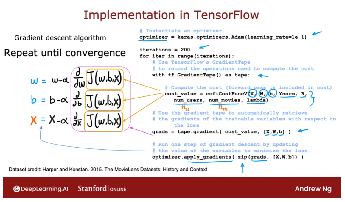
filtering algorithm TensorFlow, this is the syntax you can use.

Let’s starts with specifying
that the optimizer is keras optimizers adam with learning
rate specified here. And then for say, 200 iterations, here’s the syntax as before
with tf gradient tape, as tape, you need to provide code to compute
the value of the cost function J. So recall that in collaborative filtering, the cost function J takes is
input parameters x, w, and b as well as the ratings mean normalized.

So that’s why I’m writing y norm, r(i,j)
specifying which values have a rating, number of users or nu in our notation,
number of movies or nm in our notation or just num as well as
the regularization parameter lambda.

And if you can implement
this cost function J, then this syntax will cause TensorFlow
to figure out the derivatives for you. Then this syntax will cause TensorFlow to
record the sequence of operations used to compute the cost. And then by asking it to give
you grads equals tape.gradient, this will give you the derivative of the
cost function with respect to x, w, and b. And finally with the optimizer
that we had specified up on top, as the adam optimizer. You can use the optimizer with
the gradients that we just computed.

And does it function in python is just a
function that rearranges the numbers into an appropriate ordering for
the applied gradients function. If you are using gradient descent for
collateral filtering, recall that the cost function J would
be a function of w, b as well as x.

And if you are applying gradient descent, you take the partial
derivative respect the w. And then update w as follows. And you would also take the partial
derivative of this respect to b. And update b as follows. And similarly update
the features x as follows. And you repeat until convergence. But as I mentioned earlier
with TensorFlow and Auto Diff you’re not limited
to just gradient descent. You can also use a more powerful
optimization algorithm like the adam optimizer.

The data set you use in the practice
lab is a real data set comprising actual movies rated by actual people. This is the movie lens dataset and
it’s due to Harper and Konstan. And I hope you enjoy running this
algorithm on a real data set of movies, and ratings and see for yourself
the results that this algorithm can get.

So that’s it. That’s how you can implement
the collaborative filtering algorithm in TensorFlow. If you’re wondering why do
we have to do it this way? Why couldn’t we use a dense layer and
then model compiler and model fit? The reason we couldn’t use that old recipe
is, the collateral filtering algorithm and cost function, it doesn’t neatly
fit into the dense layer or the other standard neural network
layer types of TensorFlow. That’s why we had to implement
it this other way where we would implement the cost function ourselves.

But then use TensorFlow’s tools for
automatic differentiation, also called Auto Diff. And use TensorFlow’s implementation
of the adam optimization algorithm to let it do a lot of the work for
us of optimizing the cost function. If the model you have is a sequence
of dense neural network layers or other types of layers
supported by TensorFlow, and the old implementation recipe of
model compound model fit works.

But even when it isn’t, these tools
TensorFlow give you a very effective way to implement other learning
algorithms as well. And so I hope you enjoy playing more with
the collaborative filtering exercise in this week’s practice lab. And looks like there’s a lot of code and
lots of syntax, don’t worry about it. Make sure you have what you need to
complete that exercise successfully. And in the next video, I’d like to also
move on to discuss more of the nuances of collateral filtering and specifically the
question of how do you find related items, given one movie,
whether other movies similar to this one. Let’s go on to the next video

Finding related items

If you come to an
online shopping website and you’re looking
at a specific item, say maybe a specific book, the website may show
you things like, “Here are some other
books similar to this one” or if you’re browsing
a specific movie, it may say, “Here are some other movies
similar to this one.”

How do the websites do that?, so that when you’re
looking at one item, it gives you other similar or
related items to consider. It turns out the collaborative filtering algorithm
that we’ve been talking about gives you a nice way to find related items.
Let’s take a look. As part of the collaborative
filtering we’ve discussed, you learned features
x^(i) for every item i, for every movie i
or other type of item they’re
recommending to users. Whereas early this week, I had used a hypothetical
example of the features representing how much a movie is a romance movie
versus an action movie.

In practice, when you
use this algorithm to learn the features
x^(i) automatically, looking at the
individual features x_1, x_2, x_3, you find them to be
quite hard to interpret. Is quite hard to learn
features and say, x_1 is an action movie and x_2 is as a foreign
film and so on.

But nonetheless, these
learned features, collectively x_1, x_2, x_3, other many features, and you have collectively
these features do convey something about
what that movie is like. It turns out that given
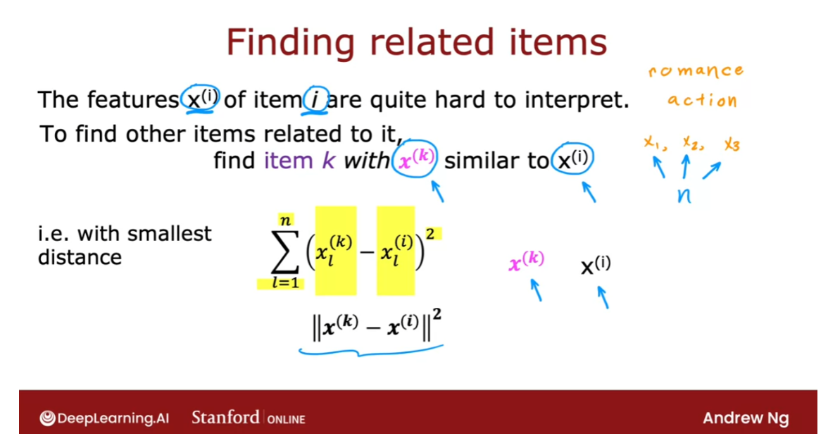
features x^(i) of item i, if you want to find other items, say other movies
related to movie i, then what you can do is try
to find the item k with features x^(k) that
is similar to x^(i).

In particular, given a
feature vector x^(k), the way we determine
what are known as similar to the feature x^(i) is as follows: is the sum from
l equals 1 through n with n features of x^(k)_l
minus x^(i)_l square. This turns out to be the
squared distance between x^(k) and x^(i) and in math, this squared distance
between these two vectors, x^(k) and x^(i), is sometimes written
as follows as well.

If you find not just
the one movie with the smallest distance between x^(k) and x^(i) but find say, the five or 10 items with the most similar
feature vectors, then you end up finding five or 10 related items
to the item x^(i). If you’re building a website
and want to help users find related products to a specific product
they are looking at, this would be a nice
way to do so because the features x^(i) give a
sense of what item i is about, other items x^(k) with similar features will turn
out to be similar to item i.

It turns out later this week, this idea of finding related items will be a small
building blocks that we’ll use to get to an even more powerful
recommended system as well.

Before wrapping up this section, I want to mention a few limitations of
collaborative filtering. In collaborative filtering, you have a set of items and so the users and the users have
rated some subset of items.

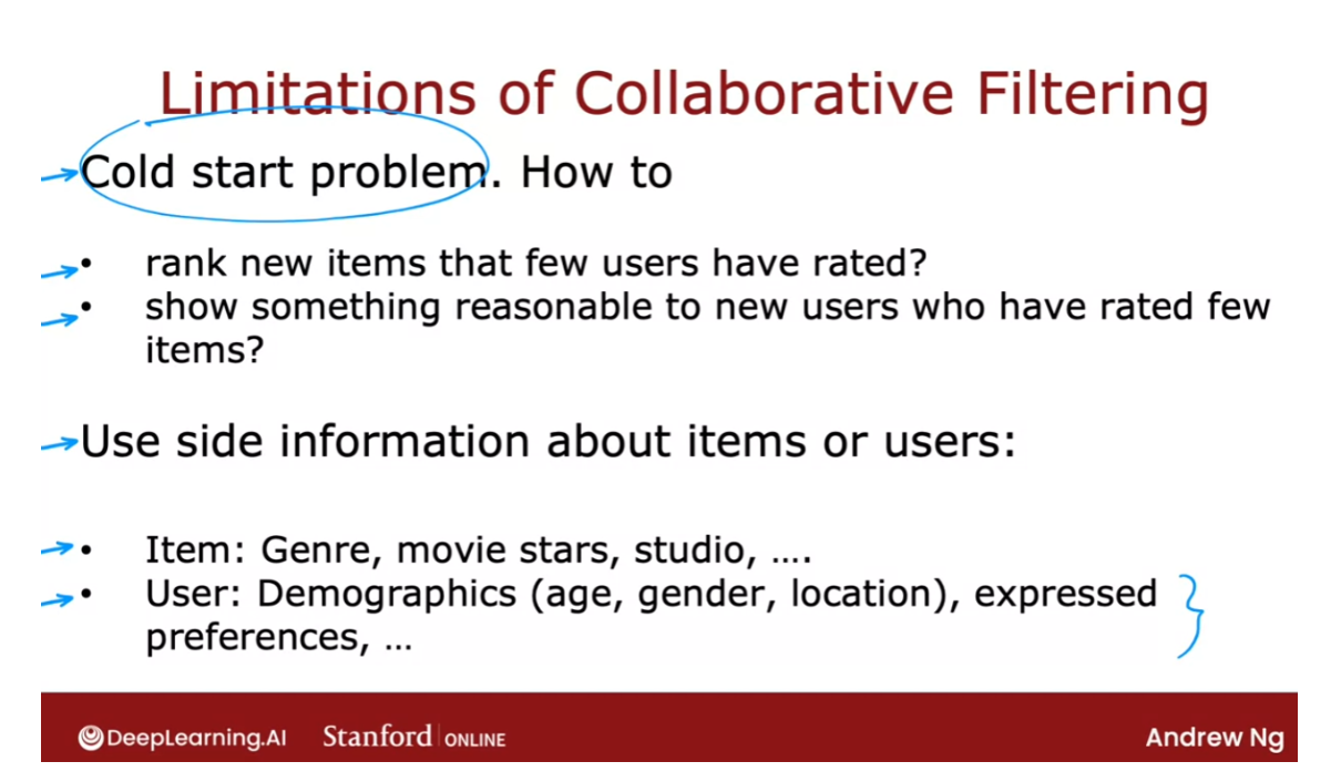
One of this
weaknesses is that is not very good at the
cold start problem. For example, if there’s a
new item in your catalog, say someone’s just
published a new movie and hardly anyone has
rated that movie yet, how do you rank the new item if very few users
have rated it before?

Similarly, for new users that have rated
only a few items, how can we make sure we show
them something reasonable? We could see in
an earlier video, how mean normalization can help with this and it
does help a lot. But perhaps even better ways to show users that rated
very few items, things that are likely
to interest them. This is called the
cold start problem, because when you
have a new item, there are few users have rated, or we have a new user that’s
rated very few items, the results of collaborative
filtering for that item or for that user may
not be very accurate.

The second limitation of collaborative filtering
is it doesn’t give you a natural way to use
side information or additional information
about items or users. For example, for a given
movie in your catalog, you might know what is
the genre of the movie, who had a movie stars, whether it is a studio, what is the budget, and so on. You may have a lot of
features about a given movie.

For a single user, you may know something
about their demographics, such as their age,
gender, location. They express preferences,
such as if they tell you they like certain
movies genres but not other movies genres, or it turns out if you know
the user’s IP address, that can tell you a lot
about a user’s location, and knowing the user’s
location might also help you guess what might the
user be interested in, or if you know whether
the user is accessing your site on a mobile
or on a desktop, or if you know what web
browser they’re using. It turns out all of these
are little cues you can get. They can be surprisingly correlated with the
preferences of a user.

It turns out by the way,
that it is known that users, that use the Chrome
versus Firefox versus Safari versus the
Microsoft Edge browser, they actually behave in
very different ways. Even knowing the user
web browser can give you a hint when you have collected enough data of what this
particular user may like.

Even though
collaborative filtering, we have multiple users give you ratings of multiple items, is a very powerful
set of algorithms, it also has some limitations. In the next video, let’s go on to develop content-based
filtering algorithms, which can address a lot
of these limitations. Content-based filtering
algorithms are a state of the art technique used in many commercial
applications today. Let’s go take a look
at how they work.

[4] Practice lab 1

Packages

We will use the now familiar NumPy and Tensorflow Packages.

import numpy as np
import tensorflow as tf
from tensorflow import keras
from recsys_utils import *

1 - Notation

General Notation	Description	Python (if any)
$r(i,j)$	scalar; = 1 if user j rated movie i = 0 otherwise
$y(i,j)$	scalar; = rating given by user j on movie i (if r(i,j) = 1 is defined)
${\mathbf{w}}^{(j)}$	vector; parameters for user j
$b^{(j)}$	scalar; parameter for user j
${\mathbf{x}}^{(i)}$	vector; feature ratings for movie i
$n_u$	number of users	num_users
$n_m$	number of movies	num_movies
$n$	number of features	num_features
$\mathbf{X}$	matrix of vectors ${\mathbf{x}}^{(i)}$	X
$\mathbf{W}$	matrix of vectors ${\mathbf{w}}^{(j)}$	W
$\mathbf{b}$	vector of bias parameters $b^{(j)}$	b
$\mathbf{R}$	matrix of elements $r(i,j)$	R

2 - Recommender Systems

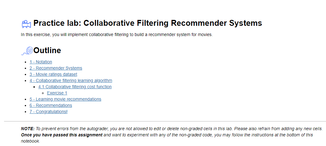
In this lab, you will implement the collaborative filtering learning algorithm and apply it to a dataset of movie ratings.
The goal of a collaborative filtering recommender system is to generate two vectors: For each user, a ‘parameter vector’ that embodies the movie tastes of a user. For each movie, a feature vector of the same size which embodies some description of the movie. The dot product of the two vectors plus the bias term should produce an estimate of the rating the user might give to that movie.

The diagram below details how these vectors are learned.

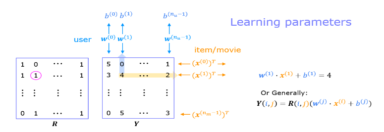
Existing ratings are provided in matrix form as shown. $Y$ contains ratings; 0.5 to 5 inclusive in 0.5 steps. 0 if the movie has not been rated. $R$ has a 1 where movies have been rated. Movies are in rows, users in columns. Each user has a parameter vector $w^{user}$ and bias. Each movie has a feature vector $x^{movie}$. These vectors are simultaneously learned by using the existing user/movie ratings as training data. One training example is shown above: ${\mathbf{w}}^{(1)}\cdot {\mathbf{x}}^{(1)}+b^{(1)}=4$. It is worth noting that the feature vector $x^{movie}$ must satisfy all the users while the user vector $w^{user}$ must satisfy all the movies. This is the source of the name of this approach - all the users collaborate to generate the rating set.

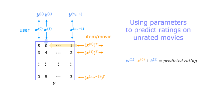
Once the feature vectors and parameters are learned, they can be used to predict how a user might rate an unrated movie. This is shown in the diagram above. The equation is an example of predicting a rating for user one on movie zero.

In this exercise, you will implement the function cofiCostFunc that computes the collaborative filtering
objective function. After implementing the objective function, you will use a TensorFlow custom training loop to learn the parameters for collaborative filtering. The first step is to detail the data set and data structures that will be used in the lab.

3 - Movie ratings dataset

The data set is derived from the MovieLens “ml-latest-small” dataset.
[F. Maxwell Harper and Joseph A. Konstan. 2015. The MovieLens Datasets: History and Context. ACM Transactions on Interactive Intelligent Systems (TiiS) 5, 4: 19:1–19:19. https://doi.org/10.1145/2827872]

The original dataset has 9000 movies rated by 600 users. The dataset has been reduced in size to focus on movies from the years since 2000. This dataset consists of ratings on a scale of 0.5 to 5 in 0.5 step increments. The reduced dataset has $n_u=443$ users, and $n_m=4778$ movies.

Below, you will load the movie dataset into the variables $Y$ and $R$.

The matrix $Y$ (a $n_m\times n_u$ matrix) stores the ratings $y^{(i,j)}$. The matrix $R$ is an binary-valued indicator matrix, where $R(i,j)=1$ if user $j$ gave a rating to movie $i$, and $R(i,j)=0$ otherwise.

Throughout this part of the exercise, you will also be working with the
matrices, $\mathbf{X}$, $\mathbf{W}$ and $\mathbf{b}$:

$$\mathbf{X}=\left[\begin{array}{c}---({\mathbf{x}}^{(0)}{)}^T---\\ ---({\mathbf{x}}^{(1)}{)}^T---\\ ⋮\\ ---({\mathbf{x}}^{(n_m-1)}{)}^T---\end{array}\right],\mathbf{W}=\left[\begin{array}{c}---({\mathbf{w}}^{(0)}{)}^T---\\ ---({\mathbf{w}}^{(1)}{)}^T---\\ ⋮\\ ---({\mathbf{w}}^{(n_u-1)}{)}^T---\end{array}\right],\mathbf{b}=\left[\begin{array}{c}{b}^{(0)}\\ b^{(1)}\\ ⋮\\ b^{(n_u-1)}\end{array}\right]$$

The $i$-th row of $\mathbf{X}$ corresponds to the
feature vector $x^{(i)}$ for the $i$-th movie, and the $j$-th row of
$\mathbf{W}$ corresponds to one parameter vector ${\mathbf{w}}^{(j)}$, for the
$j$-th user. Both $x^{(i)}$ and ${\mathbf{w}}^{(j)}$ are $n$-dimensional
vectors. For the purposes of this exercise, you will use $n=10$, and
therefore, ${\mathbf{x}}^{(i)}$ and ${\mathbf{w}}^{(j)}$ have 10 elements.
Correspondingly, $\mathbf{X}$ is a
$n_m\times 10$ matrix and $\mathbf{W}$ is a $n_u\times 10$ matrix.

We will start by loading the movie ratings dataset to understand the structure of the data.
We will load $Y$ and $R$ with the movie dataset.
We’ll also load $\mathbf{X}$, $\mathbf{W}$, and $\mathbf{b}$ with pre-computed values. These values will be learned later in the lab, but we’ll use pre-computed values to develop the cost model.

#Load data
X, W, b, num_movies, num_features, num_users = load_precalc_params_small()
Y, R = load_ratings_small()print("Y", Y.shape, "R", R.shape)
print("X", X.shape)
print("W", W.shape)
print("b", b.shape)
print("num_features", num_features)
print("num_movies",   num_movies)
print("num_users",    num_users)

Output

Y (4778, 443) R (4778, 443)
X (4778, 10)
W (443, 10)
b (1, 443)
num_features 10
num_movies 4778
num_users 443

#  From the matrix, we can compute statistics like average rating.
tsmean =  np.mean(Y[0, R[0, :].astype(bool)])
print(f"Average rating for movie 1 : {tsmean:0.3f} / 5" )

Output

Average rating for movie 1 : 3.400 / 5

4 - Collaborative filtering learning algorithm

Now, you will begin implementing the collaborative filtering learning
algorithm. You will start by implementing the objective function.

The collaborative filtering algorithm in the setting of movie
recommendations considers a set of $n$-dimensional parameter vectors
${\mathbf{x}}^{(0)},...,{\mathbf{x}}^{(n_m-1)}$, ${\mathbf{w}}^{(0)},...,{\mathbf{w}}^{(n_u-1)}$ and $b^{(0)},...,b^{(n_u-1)}$, where the
model predicts the rating for movie $i$ by user $j$ as
$y^{(i,j)}={\mathbf{w}}^{(j)}\cdot {\mathbf{x}}^{(i)}+b^{(j)}$ . Given a dataset that consists of
a set of ratings produced by some users on some movies, you wish to
learn the parameter vectors ${\mathbf{x}}^{(0)},...,{\mathbf{x}}^{(n_m-1)},{\mathbf{w}}^{(0)},...,{\mathbf{w}}^{(n_u-1)}$ and $b^{(0)},...,b^{(n_u-1)}$ that produce the best fit (minimizes
the squared error).

You will complete the code in cofiCostFunc to compute the cost
function for collaborative filtering.

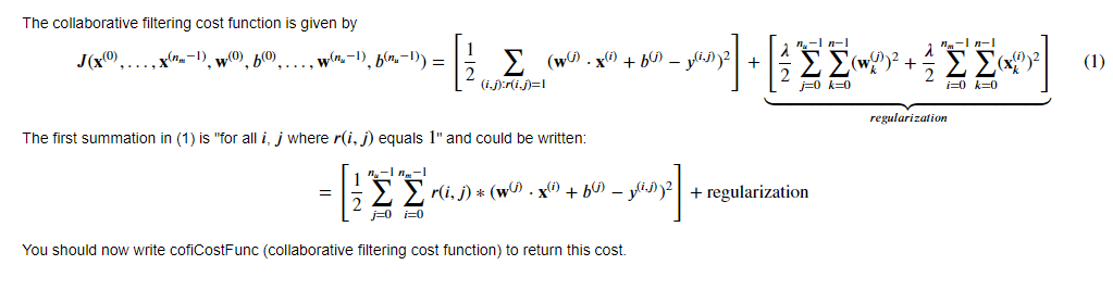
4.1 Collaborative filtering cost function

Exercise 1

For loop Implementation:
Start by implementing the cost function using for loops.
Consider developing the cost function in two steps. First, develop the cost function without regularization. A test case that does not include regularization is provided below to test your implementation. Once that is working, add regularization and run the tests that include regularization. Note that you should be accumulating the cost for user $j$ and movie $i$ only if $R(i,j)=1$.

# GRADED FUNCTION: cofi_cost_func
# UNQ_C1def cofi_cost_func(X, W, b, Y, R, lambda_):"""Returns the cost for the content-based filteringArgs:X (ndarray (num_movies,num_features)): matrix of item featuresW (ndarray (num_users,num_features)) : matrix of user parametersb (ndarray (1, num_users)            : vector of user parametersY (ndarray (num_movies,num_users)    : matrix of user ratings of moviesR (ndarray (num_movies,num_users)    : matrix, where R(i, j) = 1 if the i-th movies was rated by the j-th userlambda_ (float): regularization parameterReturns:J (float) : Cost"""nm, nu = Y.shapeJ = 0### START CODE HERE ###  for j in range(nu): # 对于用户w = W[j,:] # W的第j行： 1 x 10b_j = b[0,j]  # 第j个用户的bfor i in range(nm):  # 对于电影x = X[i,:]  # 电影特征矩阵X的第i行,代表第i部电影: 1 x 10y = Y[i,j]  # 第j个user对第i部电影的ratingsr = R[i,j]  # 用户j是否对电影i评价J += np.square(r * (np.dot(w,x) + b_j - y ) )J = J/2J += (lambda_/2) * (np.sum(np.square(W)) + np.sum(np.square(X)))    ### END CODE HERE ### return J

np.sum(np.square(W)) 是对矩阵 W 中所有元素的平方进行求和。

具体步骤如下：

1. np.square(W)：将矩阵 W 中的每个元素进行平方运算，得到一个新的矩阵，其形状与 W 相同，但每个元素都是原来元素的平方值。

2. np.sum()：对得到的平方矩阵中的所有元素进行求和，得到一个标量值。

这个操作通常用于计算矩阵中所有元素的平方和。

Hints

regularization
Regularization just squares each element of the W array and X array and them sums all the squared elements. You can utilize np.square() and np.sum().
regularization detailsJ += (lambda_/2) * (np.sum(np.square(W)) + np.sum(np.square(X)))

# Reduce the data set size so that this runs faster
num_users_r = 4
num_movies_r = 5 
num_features_r = 3X_r = X[:num_movies_r, :num_features_r]
W_r = W[:num_users_r,  :num_features_r]
b_r = b[0, :num_users_r].reshape(1,-1)
Y_r = Y[:num_movies_r, :num_users_r]
R_r = R[:num_movies_r, :num_users_r]# Evaluate cost function
J = cofi_cost_func(X_r, W_r, b_r, Y_r, R_r, 0);
print(f"Cost: {J:0.2f}")

Output

Cost: 13.67

Expected Output (lambda = 0):
13.67

# Evaluate cost function with regularization 
J = cofi_cost_func(X_r, W_r, b_r, Y_r, R_r, 1.5);
print(f"Cost (with regularization): {J:0.2f}")

Output

Cost (with regularization): 28.09

Expected Output:

28.09

Test

# Public tests
from public_tests import *
test_cofi_cost_func(cofi_cost_func)

Output

All tests passed!

Vectorized Implementation

It is important to create a vectorized implementation to compute $J$, since it will later be called many times during optimization. The linear algebra utilized is not the focus of this series, so the implementation is provided. If you are an expert in linear algebra, feel free to create your version without referencing the code below.

Run the code below and verify that it produces the same results as the non-vectorized version.

def cofi_cost_func_v(X, W, b, Y, R, lambda_):"""Returns the cost for the content-based filteringVectorized for speed. Uses tensorflow operations to be compatible with custom training loop.Args:X (ndarray (num_movies,num_features)): matrix of item featuresW (ndarray (num_users,num_features)) : matrix of user parametersb (ndarray (1, num_users)            : vector of user parametersY (ndarray (num_movies,num_users)    : matrix of user ratings of moviesR (ndarray (num_movies,num_users)    : matrix, where R(i, j) = 1 if the i-th movies was rated by the j-th userlambda_ (float): regularization parameterReturns:J (float) : Cost"""j = (tf.linalg.matmul(X, tf.transpose(W)) + b - Y)*R  # 形状： num_movies x num_usersJ = 0.5 * tf.reduce_sum(j**2) + (lambda_/2) * (tf.reduce_sum(X**2) + tf.reduce_sum(W**2))return J

对这段代码的理解

对于tf.linalg.matmul(X, tf.transpose(W)) + b中矩阵和向量相加的解释：

对于矩阵运算中矩阵和向量相加的情况，实际上是使用了广播（broadcasting）机制。

在 TensorFlow 中，如果两个张量的形状不完全相同，但是它们的形状满足一定的广播规则，那么 TensorFlow 会自动将它们扩展到相同的形状以进行逐元素的操作。对于矩阵和向量的加法，向量会自动沿着矩阵的每一行进行复制以匹配矩阵的形状，然后再执行逐元素的加法操作。

因此，在 tf.linalg.matmul(X, tf.transpose(W)) + b 中，向量 b 会被复制多次以匹配矩阵 tf.linalg.matmul(X, tf.transpose(W)) 的形状，然后再执行逐元素的加法操作。这样可以保证矩阵与向量的相加操作的正确性和效率。

让我们来确定一下这些张量的形状：

• 对于矩阵乘法 tf.linalg.matmul(X, tf.transpose(W))，假设 X 的形状为 (num_movies, num_features)，W 的形状为 (num_users, num_features)，那么乘积的形状将是 (num_movies, num_users)。

• 向量 b 的形状为 (1, num_users)。

因为广播机制会将向量 b 扩展为与矩阵相同的形状，所以在进行加法操作时，向量 b 将会沿着矩阵的第一个维度（行）复制，使其形状与矩阵相同。

因此，加法操作后得到的张量的形状将是 (num_movies, num_users)。

矩阵Z和R的形状都是num_movies x num_users，那么Z*R是什么

chatGPT回答:

当两个具有相同形状的矩阵相乘时，对应位置的元素逐个相乘。

当两个具有相同形状的矩阵相乘时，对应位置的元素逐个相乘。

在矩阵乘法中，( $Z_{ij}\times R_{ij}$ ) 的结果将会放置在 ( Z ) 和 ( R ) 相同位置的元素 ( $Z_{ij}$ ) 和 ( $R_{ij}$ ) 的对应位置上。

表达式 tf.reduce_sum(j**2) 意味着对矩阵 j 中每个元素的平方求和。

• j**2：对矩阵 j 中的每个元素进行平方运算。
• tf.reduce_sum()：对矩阵中的所有元素进行求和。

因此，tf.reduce_sum(j**2) 的结果是矩阵 j 中每个元素的平方的和。

# Evaluate cost function
J = cofi_cost_func_v(X_r, W_r, b_r, Y_r, R_r, 0);
print(f"Cost: {J:0.2f}")# Evaluate cost function with regularization 
J = cofi_cost_func_v(X_r, W_r, b_r, Y_r, R_r, 1.5);
print(f"Cost (with regularization): {J:0.2f}")

Output

Cost: 13.67
Cost (with regularization): 28.09

Expected Output:
Cost: 13.67
Cost (with regularization): 28.09

5 - Learning movie recommendations

---

After you have finished implementing the collaborative filtering cost
function, you can start training your algorithm to make
movie recommendations for yourself.

In the cell below, you can enter your own movie choices. The algorithm will then make recommendations for you! We have filled out some values according to our preferences, but after you have things working with our choices, you should change this to match your tastes.
A list of all movies in the dataset is in the file movie list.

movieList, movieList_df = load_Movie_List_pd()my_ratings = np.zeros(num_movies)          #  Initialize my ratings# Check the file small_movie_list.csv for id of each movie in our dataset
# For example, Toy Story 3 (2010) has ID 2700, so to rate it "5", you can set
my_ratings[2700] = 5 #Or suppose you did not enjoy Persuasion (2007), you can set
my_ratings[2609] = 2;# We have selected a few movies we liked / did not like and the ratings we
# gave are as follows:
my_ratings[929]  = 5   # Lord of the Rings: The Return of the King, The
my_ratings[246]  = 5   # Shrek (2001)
my_ratings[2716] = 3   # Inception
my_ratings[1150] = 5   # Incredibles, The (2004)
my_ratings[382]  = 2   # Amelie (Fabuleux destin d'Amélie Poulain, Le)
my_ratings[366]  = 5   # Harry Potter and the Sorcerer's Stone (a.k.a. Harry Potter and the Philosopher's Stone) (2001)
my_ratings[622]  = 5   # Harry Potter and the Chamber of Secrets (2002)
my_ratings[988]  = 3   # Eternal Sunshine of the Spotless Mind (2004)
my_ratings[2925] = 1   # Louis Theroux: Law & Disorder (2008)
my_ratings[2937] = 1   # Nothing to Declare (Rien à déclarer)
my_ratings[793]  = 5   # Pirates of the Caribbean: The Curse of the Black Pearl (2003)
my_rated = [i for i in range(len(my_ratings)) if my_ratings[i] > 0]print('\nNew user ratings:\n')
for i in range(len(my_ratings)):if my_ratings[i] > 0 :print(f'Rated {my_ratings[i]} for  {movieList_df.loc[i,"title"]}');

Output

New user ratings:Rated 5.0 for  Shrek (2001)
Rated 5.0 for  Harry Potter and the Sorcerer's Stone (a.k.a. Harry Potter and the Philosopher's Stone) (2001)
Rated 2.0 for  Amelie (Fabuleux destin d'Amélie Poulain, Le) (2001)
Rated 5.0 for  Harry Potter and the Chamber of Secrets (2002)
Rated 5.0 for  Pirates of the Caribbean: The Curse of the Black Pearl (2003)
Rated 5.0 for  Lord of the Rings: The Return of the King, The (2003)
Rated 3.0 for  Eternal Sunshine of the Spotless Mind (2004)
Rated 5.0 for  Incredibles, The (2004)
Rated 2.0 for  Persuasion (2007)
Rated 5.0 for  Toy Story 3 (2010)
Rated 3.0 for  Inception (2010)
Rated 1.0 for  Louis Theroux: Law & Disorder (2008)
Rated 1.0 for  Nothing to Declare (Rien à déclarer) (2010)

Now, let’s add these reviews to $Y$ and $R$ and normalize the ratings.

# Reload ratings
Y, R = load_ratings_small()# Add new user ratings to Y 
Y = np.c_[my_ratings, Y]# Add new user indicator matrix to R
R = np.c_[(my_ratings != 0).astype(int), R]# Normalize the Dataset
Ynorm, Ymean = normalizeRatings(Y, R)

Let’s prepare to train the model. Initialize the parameters and select the Adam optimizer.

#  Useful Values
num_movies, num_users = Y.shape
num_features = 100# Set Initial Parameters (W, X), use tf.Variable to track these variables
tf.random.set_seed(1234) # for consistent results
W = tf.Variable(tf.random.normal((num_users,  num_features),dtype=tf.float64),  name='W')
X = tf.Variable(tf.random.normal((num_movies, num_features),dtype=tf.float64),  name='X')
b = tf.Variable(tf.random.normal((1,          num_users),   dtype=tf.float64),  name='b')# Instantiate an optimizer.
optimizer = keras.optimizers.Adam(learning_rate=1e-1)

Let’s now train the collaborative filtering model. This will learn the parameters $\mathbf{X}$, $\mathbf{W}$, and $\mathbf{b}$.

The operations involved in learning $w$, $b$, and $x$ simultaneously do not fall into the typical ‘layers’ offered in the TensorFlow neural network package. Consequently, the flow used in Course 2: Model, Compile(), Fit(), Predict(), are not directly applicable. Instead, we can use a custom training loop.

Recall from earlier labs the steps of gradient descent.

• repeat until convergence:
  • compute forward pass
  • compute the derivatives of the loss relative to parameters
  • update the parameters using the learning rate and the computed derivatives

TensorFlow has the marvelous capability of calculating the derivatives for you. This is shown below. Within the tf.GradientTape() section, operations on Tensorflow Variables are tracked. When tape.gradient() is later called, it will return the gradient of the loss relative to the tracked variables. The gradients can then be applied to the parameters using an optimizer.
This is a very brief introduction to a useful feature of TensorFlow and other machine learning frameworks. Further information can be found by investigating “custom training loops” within the framework of interest.

iterations = 200
lambda_ = 1
for iter in range(iterations):# Use TensorFlow’s GradientTape# to record the operations used to compute the cost with tf.GradientTape() as tape:# Compute the cost (forward pass included in cost)cost_value = cofi_cost_func_v(X, W, b, Ynorm, R, lambda_)# Use the gradient tape to automatically retrieve# the gradients of the trainable variables with respect to the lossgrads = tape.gradient( cost_value, [X,W,b] )# Run one step of gradient descent by updating# the value of the variables to minimize the loss.optimizer.apply_gradients( zip(grads, [X,W,b]) )# Log periodically.if iter % 20 == 0:print(f"Training loss at iteration {iter}: {cost_value:0.1f}")

Output

Training loss at iteration 0: 2321191.3
Training loss at iteration 20: 136168.7
Training loss at iteration 40: 51863.3
Training loss at iteration 60: 24598.8
Training loss at iteration 80: 13630.4
Training loss at iteration 100: 8487.6
Training loss at iteration 120: 5807.7
Training loss at iteration 140: 4311.6
Training loss at iteration 160: 3435.2
Training loss at iteration 180: 2902.1

对tf.GradientTape()的解释：

tf.GradientTape() 是 TensorFlow 中的一个上下文管理器，用于计算梯度。在这个上下文管理器中，TensorFlow 会记录所有在其中执行的操作，以便后续计算梯度。这个功能在深度学习中特别有用，因为它允许你自动计算变量相对于某个标量的梯度。

下面是使用 tf.GradientTape() 的一般工作流程：

1. 创建一个 tf.GradientTape 上下文管理器。

2. 在 tf.GradientTape 的上下文中执行计算操作。这些操作可以是任何涉及 TensorFlow 变量的计算，例如前向传播计算、损失函数计算等。

3. 在上下文管理器结束后，调用 tape.gradient(target, sources) 方法来计算目标（通常是损失）相对于源（通常是模型参数）的梯度。

4. 计算得到的梯度可以用于更新模型参数（例如使用梯度下降算法进行优化）。

以下是使用 tf.GradientTape() 的简单示例：

import tensorflow as tf# 假设有输入 x 和参数 w
x = tf.constant(3.0)
w = tf.Variable(2.0)# 定义损失函数
def loss_fn(w, x):return w * x**2# 创建一个 tf.GradientTape 上下文管理器
with tf.GradientTape() as tape:# 在上下文中执行计算loss = loss_fn(w, x)# 计算损失相对于参数 w 的梯度
grad = tape.gradient(loss, w)
print("Gradient of loss with respect to w:", grad.numpy())

在这个示例中，loss 是基于参数 w 和输入 x 计算得到的损失函数值。使用 tf.GradientTape() 记录了计算 loss 过程中涉及的所有操作，并计算了损失相对于参数 w 的梯度。最后，打印出了损失相对于参数 w 的梯度值。

在这个代码片段中，optimizer.apply_gradients(zip(grads, [X, W, b])) 通过 zip() 函数将梯度与相应的变量组合在一起，然后将它们传递给优化器 optimizer 的 apply_gradients() 方法。

• grads 是梯度的列表，其中每个梯度与对应的变量（X、W 和 b）一一对应。这意味着 grads 的第一个梯度对应于 X，第二个梯度对应于 W，第三个梯度对应于 b。

• [X, W, b] 是包含要更新的变量的列表。

• zip(grads, [X, W, b]) 将每个变量的梯度与对应的变量一一对应地打包在一起，形成一个元组的列表。

• optimizer.apply_gradients() 方法接受这个打包好的梯度和变量的元组列表，并使用这些梯度来更新相应的变量。

通过具体例子解释：zip(grads, [X, W, b])

假设我们有以下变量和梯度：

• X 是一个张量，表示某个神经网络中的输入；
• W 是一个张量，表示神经网络的权重；
• b 是一个张量，表示神经网络的偏置；
• grad_X 是 X 相对于某个损失函数的梯度；
• grad_W 是 W 相对于损失函数的梯度；
• grad_b 是 b 相对于损失函数的梯度。

我们有如下代码：

import tensorflow as tf# 假设我们有变量 X、W、b 和它们的梯度 grad_X、grad_W、grad_b
X = tf.Variable([1.0, 2.0, 3.0])
W = tf.Variable([0.1, 0.2, 0.3])
b = tf.Variable(0.5)
grad_X = tf.constant([0.1, 0.2, 0.3])
grad_W = tf.constant([0.01, 0.02, 0.03])
grad_b = tf.constant(0.05)# 创建优化器
optimizer = tf.optimizers.SGD(learning_rate=0.1)# 打包梯度和变量
grads = [grad_X, grad_W, grad_b]
variables = [X, W, b]
grads_and_vars = zip(grads, variables)# 使用优化器应用梯度
optimizer.apply_gradients(grads_and_vars)

在这个例子中，我们将 grad_X、grad_W 和 grad_b 与对应的变量 X、W 和 b 组合在一起，形成一个包含了梯度和变量的元组列表。这个操作使用了 zip(grads, variables)。

最后，优化器 optimizer 将应用这些梯度来更新相应的变量 X、W 和 b。

在这个例子中，zip(grads, variables) 的结果是一个迭代器，它将 grads 和 variables 中对应位置的元素依次打包成元组。

具体来说，对于给定的 grads 和 variables，zip(grads, variables) 的结果如下：

[(grad_X, X),(grad_W, W),(grad_b, b)
]

这样，每个元组中的第一个元素是梯度（grad_X, grad_W, grad_b），第二个元素是对应的变量（X, W, b）。

6 - Recommendations

Below, we compute the ratings for all the movies and users and display the movies that are recommended. These are based on the movies and ratings entered as my_ratings[] above. To predict the rating of movie $i$ for user $j$, you compute ${\mathbf{w}}^{(j)}\cdot {\mathbf{x}}^{(i)}+b^{(j)}$. This can be computed for all ratings using matrix multiplication.

# Make a prediction using trained weights and biases
p = np.matmul(X.numpy(), np.transpose(W.numpy())) + b.numpy()#restore the mean
pm = p + Ymeanmy_predictions = pm[:,0]# sort predictions
ix = tf.argsort(my_predictions, direction='DESCENDING')for i in range(17):j = ix[i]if j not in my_rated:print(f'Predicting rating {my_predictions[j]:0.2f} for movie {movieList[j]}')print('\n\nOriginal vs Predicted ratings:\n')
for i in range(len(my_ratings)):if my_ratings[i] > 0:print(f'Original {my_ratings[i]}, Predicted {my_predictions[i]:0.2f} for {movieList[i]}')

Output

Predicting rating 4.49 for movie My Sassy Girl (Yeopgijeogin geunyeo) (2001)
Predicting rating 4.48 for movie Martin Lawrence Live: Runteldat (2002)
Predicting rating 4.48 for movie Memento (2000)
Predicting rating 4.47 for movie Delirium (2014)
Predicting rating 4.47 for movie Laggies (2014)
Predicting rating 4.47 for movie One I Love, The (2014)
Predicting rating 4.46 for movie Particle Fever (2013)
Predicting rating 4.45 for movie Eichmann (2007)
Predicting rating 4.45 for movie Battle Royale 2: Requiem (Batoru rowaiaru II: Chinkonka) (2003)
Predicting rating 4.45 for movie Into the Abyss (2011)Original vs Predicted ratings:Original 5.0, Predicted 4.90 for Shrek (2001)
Original 5.0, Predicted 4.84 for Harry Potter and the Sorcerer's Stone (a.k.a. Harry Potter and the Philosopher's Stone) (2001)
Original 2.0, Predicted 2.13 for Amelie (Fabuleux destin d'Amélie Poulain, Le) (2001)
Original 5.0, Predicted 4.88 for Harry Potter and the Chamber of Secrets (2002)
Original 5.0, Predicted 4.87 for Pirates of the Caribbean: The Curse of the Black Pearl (2003)
Original 5.0, Predicted 4.89 for Lord of the Rings: The Return of the King, The (2003)
Original 3.0, Predicted 3.00 for Eternal Sunshine of the Spotless Mind (2004)
Original 5.0, Predicted 4.90 for Incredibles, The (2004)
Original 2.0, Predicted 2.11 for Persuasion (2007)
Original 5.0, Predicted 4.80 for Toy Story 3 (2010)
Original 3.0, Predicted 3.00 for Inception (2010)
Original 1.0, Predicted 1.41 for Louis Theroux: Law & Disorder (2008)
Original 1.0, Predicted 1.26 for Nothing to Declare (Rien à déclarer) (2010)

In practice, additional information can be utilized to enhance our predictions. Above, the predicted ratings for the first few hundred movies lie in a small range. We can augment the above by selecting from those top movies, movies that have high average ratings and movies with more than 20 ratings. This section uses a Pandas data frame which has many handy sorting features.

filter=(movieList_df["number of ratings"] > 20)
movieList_df["pred"] = my_predictions
movieList_df = movieList_df.reindex(columns=["pred", "mean rating", "number of ratings", "title"])
movieList_df.loc[ix[:300]].loc[filter].sort_values("mean rating", ascending=False)

Output

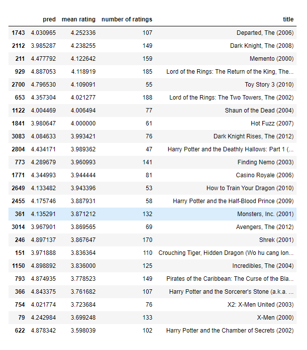
7 - Congratulations!

You have implemented a useful recommender system!

Grades

[5] Practice quiz: Recommender systems implementation

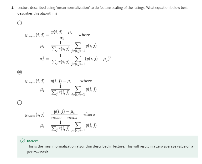
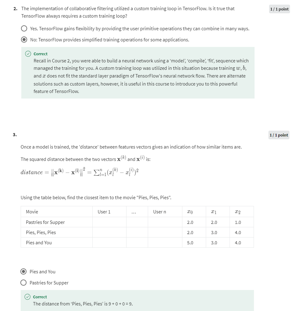
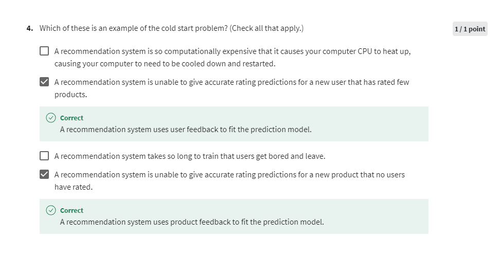
[6] Content-based filtering

Collaborative filtering vs Content-based filtering

In this video, we’ll start
to develop a second type of recommender system called a content-based
filtering algorithm. To get started, let’s
compare and contrast the collaborative filtering
approach that we’ll be looking at so far with this new content-based
filtering approach.

• 协同过滤算法：基于用户之间的相似性或项目之间的相似性来进行推荐。它会分析用户对项目的评分数据，找出具有相似评分模式的用户或项目，并根据这种相似性来推荐新的项目给用户。
• 基于内容的过滤算法：基于项目或用户的特征来进行推荐。它会分析项目和用户的特征，例如项目的关键词、类别、描述，以及用户的偏好、历史行为等，然后通过匹配项目和用户的特征来进行推荐。

Let’s take a look. With collaborative filtering, the general approach is that
we would recommend items to you based on ratings of users who gave similar
ratings as you. We have some number of users give some ratings
for some items, and the algorithm
figures out how to use that to recommend
new items to you.

In contrast, content-based
filtering takes a different approach to deciding what to
recommend to you. A content-based
filtering algorithm will recommend items
to you based on the features of users and features of the items
to find a good match. In other words, it requires having some
features of each user, as well as some features of each item and it uses
those features to try to decide which items and users might be a good
match for each other.

With a content-based
filtering algorithm, you still have data where
users have rated some items. Well, content-based filtering will continue to use r, i, j to denote whether
or not user j has rated item i and will
continue to use y i, j to denote the rating that user j is given
item i if it’s defined.

But the key to content-based filtering is that we will be able to
make good use of features of the user
and of the items to find better matches than potentially a pure collaborative filtering approach
might be able to.

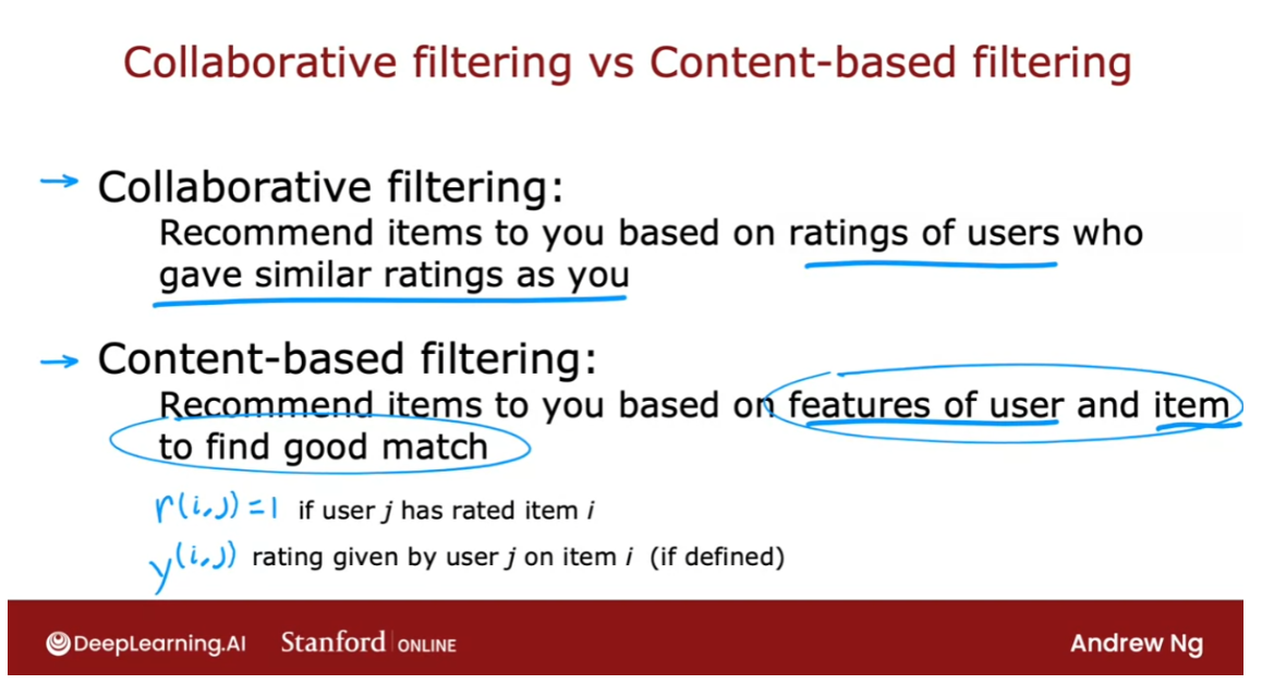
Let’s take a look
at how this works. In the case of movie
recommendations, here are some
examples of features. You may know the
age of the user, or you may have the
gender of the user. This could be a one-hot feature similar to what you saw
when we were talking about decision trees where you could have a one-hot
feature with the values based on whether the user’s
self-identified gender is male or female or unknown, and you may know the
country of the user. If there are about 200 countries in the world then also be a one-hot feature with
about 200 possible values.

You can also look at
past behaviors of the user to construct
this feature vector. For example, if you look at the top thousand movies
in your catalog, you might construct a thousand
features that tells you of the thousand most
popular movies in the world which of these
has the user watch. In fact, you can also take
ratings the user might have already given in order
to construct new features.

It turns out that if you
have a set of movies and if you know what
genre each movie is in, then the average rating per genre that the
user has given. Of all the romance movies
that the user has rated, what was the average rating? Of all the action movies
that the user has rated, what was the average rating? And so on for all
the other genres. This too can be a powerful
feature to describe the user. One interesting thing about
this feature is that it actually depends on the ratings
that the user had given. But there’s nothing
wrong with that.

Constructing a
feature vector that depends on the user’s ratings is a completely fine way to develop a feature vector
to describe that user. With features like these
you can then come up with a feature vector
x subscript u, use as a user superscript
j for user j.

Similarly, you can also
come up with a set of features for each
movie of each item, such as what was the
year of the movie? What’s the genre or genres
of the movie of known? If there are critic
reviews of the movie, you can construct one
or multiple features to capture something about what the critics are saying
about the movie.

Or once again, you
can actually take user ratings of the movie
to construct a feature of, say, the average
rating of this movie. This feature again
depends on the ratings that users are given but again, does nothing wrong with that. You can construct a feature for a given movie that depends on the ratings
that movie had received, such as the average
rating of the movie. Or if you wish,
you can also have average rating per country or average rating per user
demographic as they want to construct other types of features of the movies as well.

With this, for each movie, you can then construct
a feature vector, which I’m going to
denote x subscript m, m stands for movie, and superscript i for movie i. Given features like this, the task is to try to
figure out whether a given movie i is going to
be good match for user j.

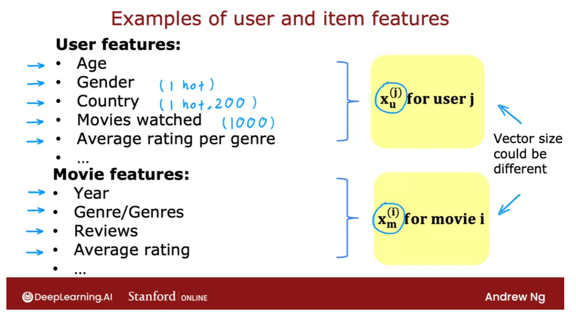
Notice that the
user features and movie features can be
very different in size. For example, maybe the
user features could be 1500 numbers and
the movie features could be just 50 numbers. That’s okay too. In
content-based filtering, we’re going to develop an
algorithm that learns to match users and movies.

Previously, we were predicting the rating of user j on movie i as wj dot products
of xi plus bj. In order to develop
content-based filtering, I’m going to get rid of bj. It turns out this won’t hurt the performance of the
content-based filtering at all. Instead of writing wj for a
user j and xi for a movie i, I’m instead going to just replace this notation with vj_u. This v here stands for a vector.

There’ll be a list of
numbers computed for user j and the u subscript
here stands for user. Instead of xi, I’m going to compute a
separate vector subscript m, to stand for the movie and for movie is what a
superscript stands for. Vj_u as a vector as
a list of numbers computed from the
features of user j and vi_m is a list of
numbers computed from the features like
the ones you saw on the previous slide of movie i.

If we’re able to come up with an appropriate choice
of these vectors, vj_u and vi_m, then hopefully the dot product between these two
vectors will be a good prediction of the rating that user
j gives movie i. Just illustrate what
a learning algorithm could come up with.

If v, u, that is a user vector, turns out to capture
the user’s preferences, say is 4.9, 0.1, and so on. Lists of numbers like that. The first number captures how much do they
like romance movies. Then the second number
captures how much do they like action movies and so on. Then v_m, the movie
vector is 4.5, 0.2, and so on and so forth
of these numbers capturing how much is
this a romance movie, how much is this an
action movie, and so on.

Then the dot product, which multiplies these lists of numbers element-wise
and then takes a sum, hopefully, will give
a sense of how much this particular user will
like this particular movie. The challenges given features
of a user, say xj_u, how can we compute
this vector vj_u that represents succinctly or compactly the
user’s preferences? Similarly given
features of a movie, how can we compute vi_m?

Notice that whereas x_u and x_m could be
different in size, one could be very long
lists of numbers, one could be much shorter list, v here have to be the same size. Because if you want to take a dot product
between v_u and v_m, then both of them have to have the same dimensions such as maybe both of these
are say 32 numbers.

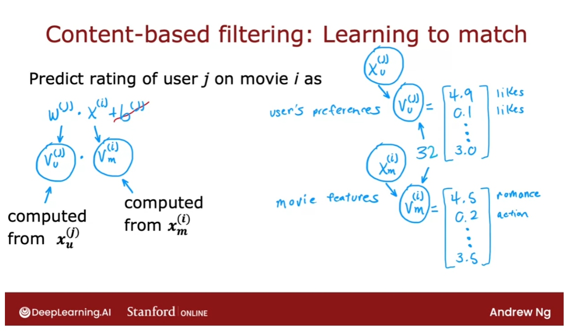
总结一下，在协同过滤中，我们有许多用户对不同的项目进行评分。

相比之下，在基于内容的过滤中，我们有用户的特征和项目的特征，并且我们想找到一种方法来找到用户和项目之间的良好匹配关系。我们将要做的是计算这些向量，对于用户是 v_u，对于项目是 v_m，覆盖了电影，然后对它们进行点乘，以尝试找到良好的匹配项。

To summarize, in
collaborative filtering, we had number of users give
ratings of different items. In contrast, in
content-based filtering, we have features of users
and features of items and we want to find a way to find good matches between the
users and the items. The way we’re going to do so
is to compute these vectors, v_u for the users and v_m for
the items over the movies, and then take dot
products between them to try to
find good matches.

How do we compute
the v_u and v_m? Let’s take a look at
that in the next video.

Deep learning for content-based filtering

A good way to develop a content-based
filtering algorithm is to use deep learning. The approach you see in
this video is the way that many important commercial state-of-the-art content-based
filtering algorithms are built today.
Let’s take a look.

Recall that in our approach, given a feature vector
describing a user, such as age and
gender, and country, and so on, we have to compute the vector v_u, and similarly, given a vector describing a movie such as year of release, the stars in the
movie, and so on, we have to compute a vector v_m.

In order to do the former, we’re going to use
a neural network. The first neural network will be what we’ll call
the user network. Here’s an example
of user network, that takes as input the list of features of the user, x_u, so the age, the gender, the country of the
user, and so on. Then using a few layers, say dense neural network layers, it will output this vector
v_u that describes the user.

Notice that in this
neural network, the output layer has 32 units, and so v_u is actually
a list of 32 numbers. Unlike most of the
neural networks that we were using earlier, the final layer is not
a layer with one unit, it’s a layer with 32 units.

Similarly, to compute
v_m for a movie, we can have a movie
network as follows, that takes as input
features of the movie and through a few layers of a neural network
is outputting v_m, that vector that
describes the movie.

Finally, we’ll predict the
rating of this user on that movie as v_ u
dot product with v_m. Notice that the user network
and the movie network can hypothetically have
different numbers of hidden layers and
different numbers of units per hidden layer. All the output layer needs to have the same size of
the same dimension.

In the description
you’ve seen so far, we were predicting the 1-5
or 0-5 star movie rating. If we had binary labels, if y was to the user
like or favor an item, then you can also modify
this algorithm to output. Instead of v_u.v_m, you can apply the
sigmoid function to that and use this to predict the probability
that’s y^i,j is 1.

To flesh out this notation, we can also add
superscripts i and j here if we want
to emphasize that this is the prediction
by user j on movie i. I’ve drawn here
the user network and the movie network as two
separate neural networks.

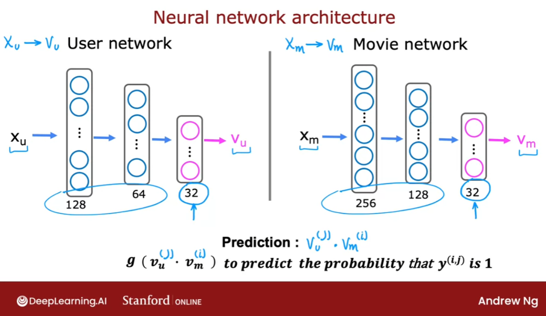
But it turns out
that we can actually draw them together in a single diagram as if it
was a single neural network. This is what it looks like. On the upper portion
of this diagram, we have the user network which inputs x_u and ends
up computing v_u. On the lower portion
of this diagram, we have what was
the movie network, the input is x_m and
ends up computing v_m, and these two vectors are
then dot-product together. This dot here
represents dot product, and this gives us
our prediction.

Now, this model has
a lot of parameters. Each of these layers of
a neural network has a usual set of parameters
of the neural network. How do you train all
the parameters of both the user network
and the movie network? What we’re going to do is
construct a cost function J, which is going to
be very similar to the cost function that you saw in collaborative filtering, which is assuming
that you do have some data of some users
having rated some movies, we’re going to sum
over all pairs i and j of where you have labels, where i,j equals 1 of the difference
between the prediction.

That would be v_u^j
dot product with v_m^i minus y^ij squared. The way we would
train this model is depending on the parameters
of the neural network, you end up with
different vectors here for the users
and for the movies.

What we’d like to do is
train the parameters of the neural network
so that you end up with vectors for the users and for
the movies that results in small squared error into
predictions you get out here. To be clear, there’s no separate training procedure for the user and movie networks. This expression down here, this is the cost
function used to train all the parameters of the
user and the movie networks.

We’re going to judge the two
networks according to how well v_u and v_m predict y^ij, and with this cost function, we’re going to use
gradient descent or some other optimization
algorithm to tune the parameters of the
neural network to cause the cost function J to
be as small as possible. If you want to
regularize this model, we can also add the usual neural network regularization term to encourage the neural
networks to keep the values of their
parameters small.

It turns out, after you’ve
trained this model, you can also use this
to find similar items. This is akin to
what we have seen with collaborative
filtering features, helping you find similar items as well.

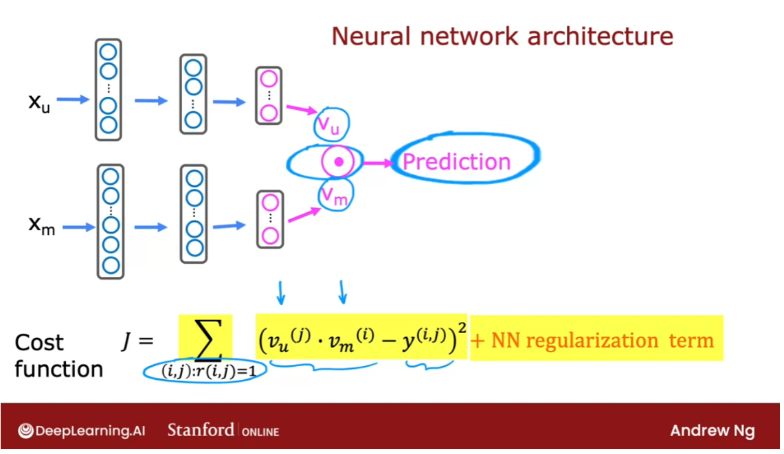
Let’s take a look. V_u^j is a vector of
length 32 that describes a user j that have
features x_ u^j. Similarly, v^i_m is a vector of length 32 that describes a movie with these
features over here.

Given a specific movie, what if you want to find
other movies similar to it? Well, this vector v^i_m
describes the movie i. If you want to find other
movies similar to it, you can then look for other
movies k so that the distance between the vector describing movie k and the vector
describing movie i, that the squared
distance is small.

This expression plays
a role similar to what we had previously with
collaborative filtering, where we talked about finding
a movie with features x^k that was similar
to the features x^i. Thus, with this approach, you can also find items
similar to a given item.

One final note, this can be
pre-computed ahead of time. By that I mean, you can run a compute
server overnight to go through the list of all your movies and
for every movie, find similar movies to
it, so that tomorrow, if a user comes to
the website and they’re browsing
a specific movie, you can already have
pre-computed to 10 or 20 most similar movies to show to the
user at that time.

The fact that you can
pre-compute ahead of time what’s similar
to a given movie, will turn out to be important later when we talk about scaling up this approach to a very
large catalog of movies. That’s how you can use
deep learning to build a content-based
filtering algorithm.

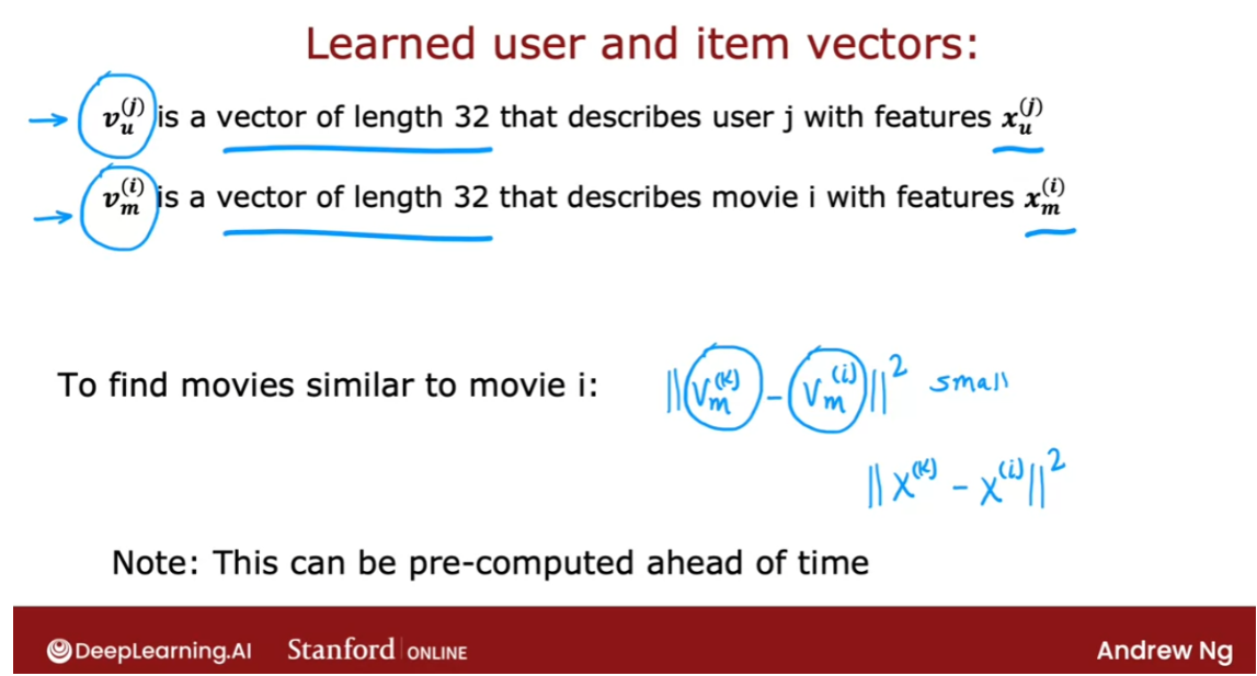
You might remember when we were talking about
decision trees and the pros and cons of decision trees versus
neural networks. I mentioned that one
of the benefits of neural networks is that
it’s easier to take multiple neural networks and put them together to make them work in concert to
build a larger system. What you just saw was
actually an example of that, where we could take
a user network and the movie network and
put them together, and then take the inner
product of the outputs.

This ability to put two neural networks
together this how we’ve managed to come up with a more complex architecture that turns out to
be quite powerful. One notes, if you’re implementing these
algorithms in practice, I find that developers often end up spending a lot
of time carefully designing the features
needed to feed into these content-based
filtering algorithms.

If we end up building one of
these systems commercially, it may be worth
spending some time engineering good features for
this application as well. In terms of these applications, one limitation
that the algorithm as we’ve described
it is it can be computationally very
expensive to run if you have a large catalog of a lot of different movies you
may want to recommend.

In the next video, let’s
take a look at some of the practical issues
and how you can modify this algorithm to make it
scale that are working on even very large
item catalogs. Let’s go see that
in the next video.

Recommending from a large catalogue

Today’s recommender systems will sometimes
need to pick a handful of items to recommend. From a catalog of thousands or millions or
10s of millions or even more items. How do you do this efficiently
computationally, let’s take a look.

Here’s in your network we’ve been using to make predictions about
how a user might rate an item. Today a large movie streaming site
may have thousands of movies or a system that is trying to
decide what ad to show. May have a catalog of millions
of ads to choose from. Or a music streaming sites may have 10s
of millions of songs to choose from. And large online shopping
sites can have millions or even 10s of millions of
products to choose from.

When a user shows up on your website,
they have some feature Xu. But if you need to take thousands
of millions of items to feed through this neural network in
order to compute in the product. To figure out which products
you should recommend, then having to run neural
network inference.

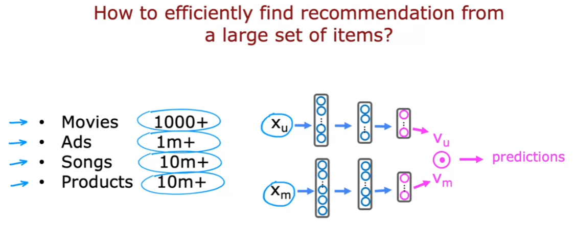
Thousands of millions of times every
time a user shows up on your website becomes computationally infeasible. Many law scale recommender
systems are implemented as two steps which are called the retrieval and
ranking steps.

The idea is during the retrieval
step will generate a large list of plausible item candidates. That tries to cover a lot of possible
things you might recommend to the user and it’s okay during the retrieval step. If you include a lot of items that
the user is not likely to like and then during the ranking
step will fine tune and pick the best items to
recommend to the user.

So here’s an example, during the retrieval
step we might do something like. For each of the last 10
movies that the user has watched find the 10 most similar movies. So this means for
example if a user has watched the movie I with vector VIM
you can find the movies hey with vector VKM that
is similar to that. And as you saw in the last video
finding the similar movies, the given movie can be pre computed.

So having pre computed the most
similar movies to give a movie, you can just pull up the results
using a look up table. This would give you an initial set of
maybe somewhat plausible movies to recommend to user that just
showed up on your website.

Additionally you might
decide to add to it for whatever are the most viewed
three genres of the user. Say that the user has watched
a lot of romance movies and a lot of comedy movies and
a lot of historical dramas. Then we would add to the list of
possible item candidates the top 10 movies in each of these three genres.

And then maybe we will also
add to this list the top 20 movies in the country of the user. So this retrieval step can
be done very quickly and you may end up with a list of 100 or
maybe 100s of plausible movies. To recommend to the user and hopefully this list will
recommend some good options. But it’s also okay if it includes some
options that the user won’t like at all. The goal of the retrieval step
is to ensure broad coverage to have enough movies at least
have many good ones in there.

Finally, we would then take all the items
we retrieve during the retrieval step and combine them into a list. Removing duplicates and removing items
that the user has already watched or that the user has already purchased and that you may not want to
recommend to them again.

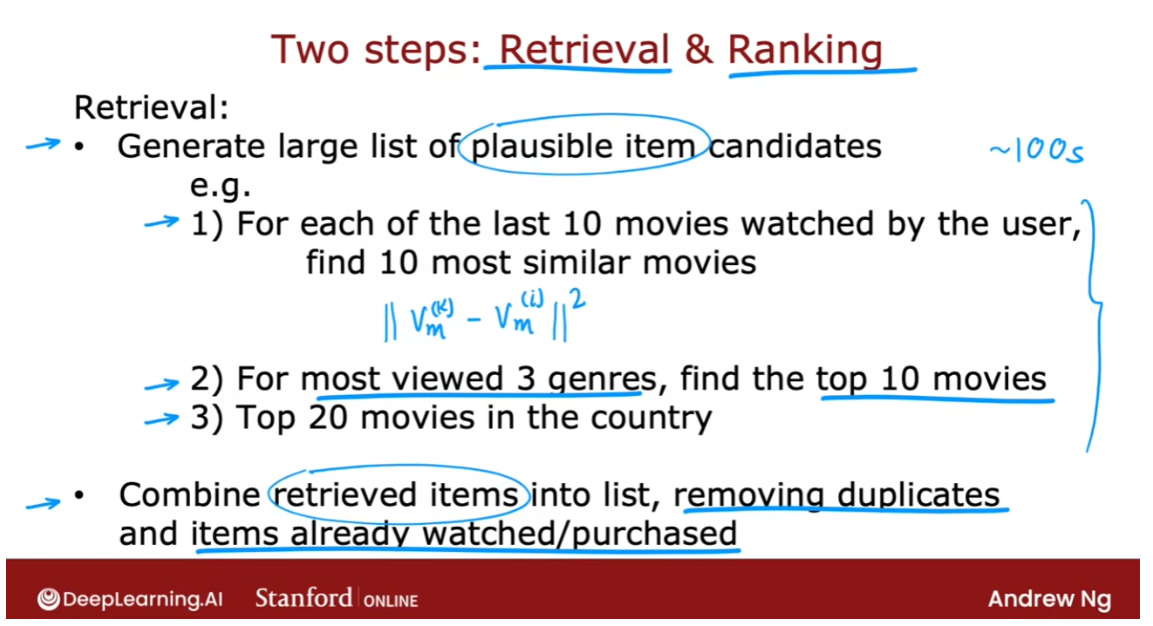
The second step of this
is then the ranking step. During the ranking step you will take the
list retrieved during the retrieval step. So this may be just hundreds
of possible movies and rank them using the learned model. And what that means is you will
feed the user feature vector and the movie feature actor
into this neural network. And for each of the user movie
pairs compute the predicted rating. And based on this, you now have
all of the say 100 plus movies, the ones that the user is most
likely to give a high rating to.

And then you can just display the rank
list of items to the user depending on what you think the user will give. The highest rating to one
additional optimization is that if you have computed VM. For all the movies in advance,
then all you need to do is to do inference on this part of the neural network
a single time to compute VU. And then take that VU they just computed
for the user on your website right now. And take the inner product between VU and
VM.

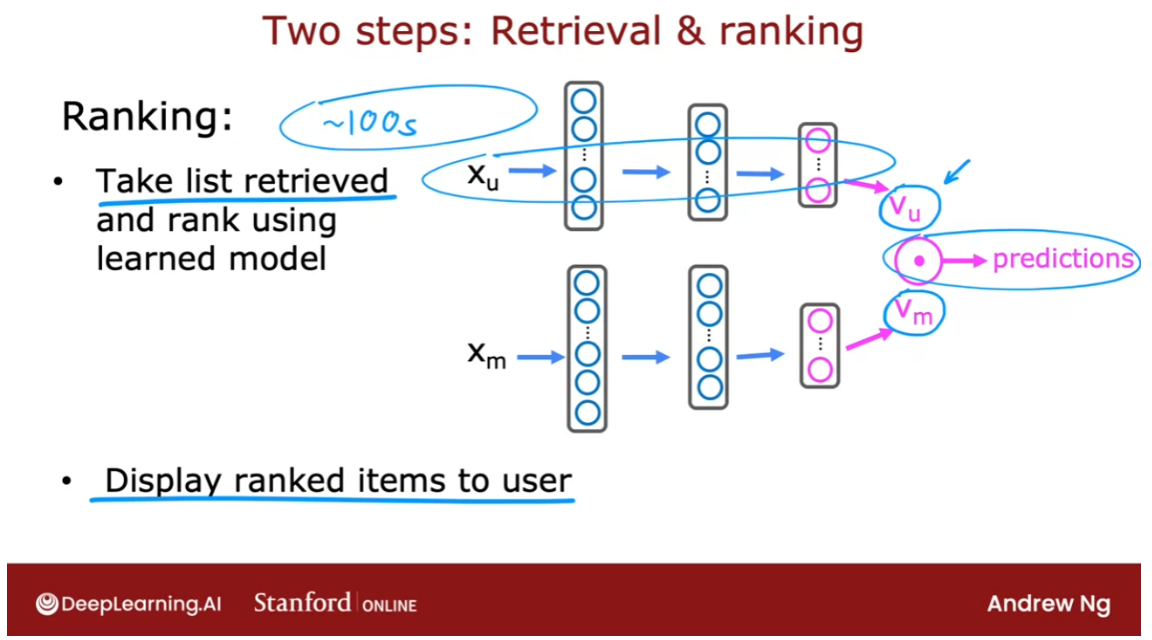
For the movies that you have
retrieved during the retrieval step. So this computation can be
done relatively quickly. If the retrieval step just
brings up say 100s of movies, one of the decisions you need to make for this algorithm is how many items do you want
to retrieve during the retrieval step? To feed into the more
accurate ranking step.

During the retrieval step, retrieving more items will tend
to result in better performance. But the algorithm will end up
being slower to analyze or to optimize the trade off between
how many items to retrieve to retrieve 100 or 500 or 1000 items.

I would recommend carrying out offline
experiments to see how much retrieving additional items results in
more relevant recommendations. And in particular,
if the estimated probability that YIJ. Is equal to one according to
your neural network model. Or if the estimated rating of Y
being high of the retrieve items according to your model’s prediction
ends up being much higher.

If only you were to retrieve say 500
items instead of only 100 items, then that would argue for
maybe retrieving more items. Even if it slows down the algorithm a bit. But with the separate retrieval step and
the ranking step, this allows many recommender systems today to give
both fast as well as accurate results.

Because the retrieval step tries to
prune out a lot of items that are just not worth doing the more detailed
influence and inner product on. And then the ranking step makes
a more careful prediction for what are the items that the user is
actually likely to enjoy so that’s it.

This is how you make your
recommender system work efficiently even on very large catalogs of movies or
products or what have you.

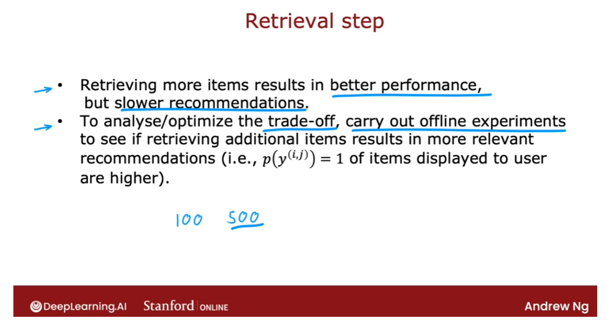
Now, it turns out that as commercially
important as our recommender systems, there are some significant ethical
issues associated with them as well. And unfortunately there have been
recommender systems that have created harm. So as you build your
own recommender system, I hope you take an ethical approach and
use it to serve your users. And society as large as
well as yourself and the company that you might be working for. Let’s take a look at the ethical issues
associated with recommender systems in the next video

Ethical use of recommender systems

Even though recommender
systems have been very profitable for some
businesses, that happens, some use cases that have left people and society
at large worse off. However, you use
recommender systems or for that matter other
learning algorithms, I hope you only do
things that make society at large and
people better off.

Let’s take a look at some of the problematic use cases
of recommender systems, as well as ameliorations to reduce harm or to increase the amount of
good that they can do. As you’ve seen in
the last few videos, there are many ways of
configuring a recommender system.

When we saw binary labels, the label y could be, does a user engage
or did they click or did they explicitly
like an item? When designing a
recommender system, choices in setting the goal
of the recommender system and a lot of choices and deciding what to
recommend to users.

For example, you can
decide to recommend to users movies most likely to be rated five stars by that
user. That seems fine. That seems like a
fine way to show users movies that
they would like. Or maybe you can recommend to the user products that they
are most likely to purchase. That seems like a
very reasonable use of a recommender system as well. Versions of recommender
systems can also be used to decide what
ads to show to a user.

One thing you could do is
to recommend or really to show to the user ads that are most
likely to be clicked on. Actually, what many
companies will do is try to show ads that are
likely to be clicked on and where the
advertiser had put in a high bid because
for many ad models, the revenue that the company collects depends on
whether the ad was clicked on and what the
advertiser had bid per-click.

While this is a
profit-maximizing strategy, there are also some possible
negative implications of this type of advertising. I’ll give a specific
example on the next slide. One other thing that
many companies do is try to recommend products that generate the largest profit.

If you go to a website and
search for a product today, there are many websites
that are not showing you the most relevant
product or the product that you are most
likely to purchase. But is instead
trying to show you the products that will generate the largest profit
for the company. If a certain product is
more profitable for them, because they can buy it more cheaply and sell it
at a higher price, that gets ranked higher
in the recommendations.

Now, many companies view a
pressure to maximize profit. This doesn’t seem like an unreasonable thing to
do but on the flip side, from the user perspective, when a website recommends
to you a product, sometimes it feels
it could be nice if the website was transparent with you about the criteria by which it is deciding
what to show you.

Is it trying to maximize
their profits or trying to show you things
that are most useful to you? On video websites or
social media websites, a recommender system can also
be modified to try to show you the content that leads
to the maximum watch time. Specifically, websites that are an ad revenue tend to have an incentive to keep you on
the website for a long time. Trying to maximize the time you spend on the site is one way for the site to try to get more of your time so they can
show you more ads.

Recommender systems today
are used to try to maximize user engagement or to
maximize the amount of time that someone spends on
a site or a specific app. Whereas the first two of
these seem quite innocuous, the third, fourth, and fifth, they may be just fine. They may not cause
any harm at all. Or they could also be problematic use cases
for recommender systems.

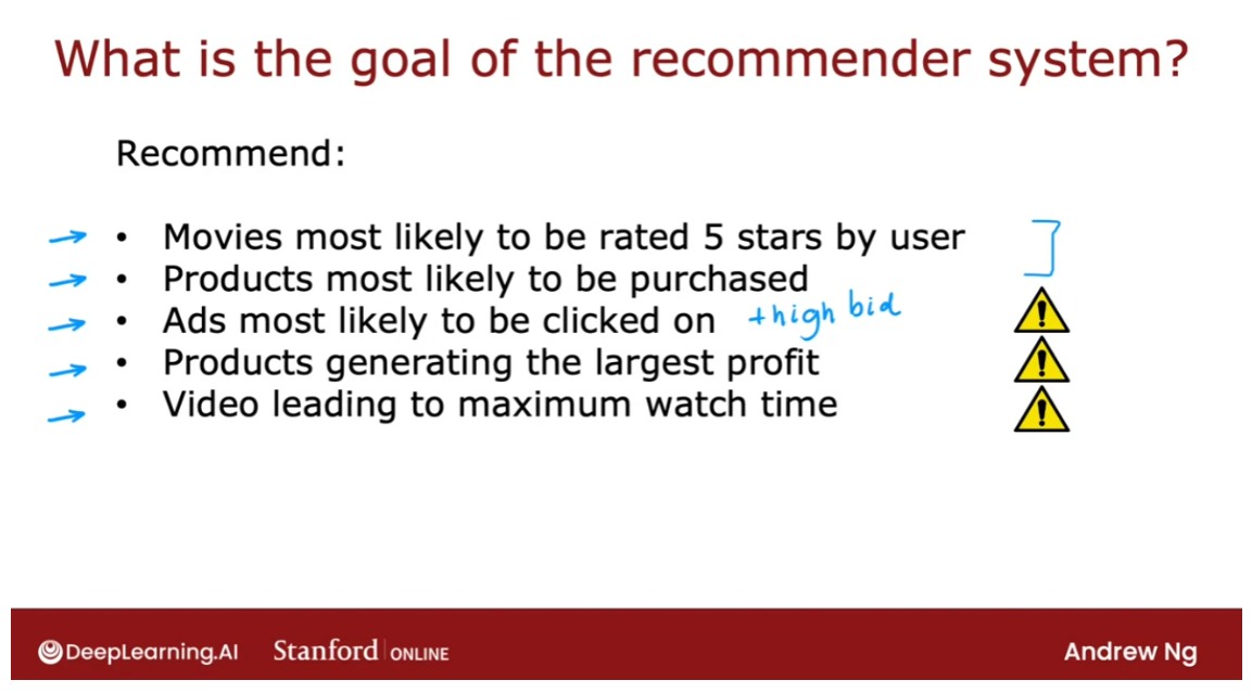
Let’s take a deeper
look at some of these potentially
problematic use cases. Let me start with the
advertising example. It turns out that
the advertising industry can sometimes be an amplifier of some of the
most harmful businesses. They can also be an
amplifier of some of the best and the most
fruitful businesses. Let me illustrate with a good
example and a bad example.

Take the travel industry. I think in the travel industry, the way to succeed is to try to give good travel
experiences to users, to really try to serve users. Now it turns out that if there’s a really good travel company, they can sell you a trip to fantastic destinations and make sure you and your friends and
family have a lot of fun. Then a good travel business, I think will often end up
being more profitable. The other business
is more profitable. They can then bid
higher for ads. It can afford to pay
more to get users. Because it can afford
to bid higher for ads an online advertising
site will show its ads more often and drive more users to this good company.

This is a virtuous cycle where the more users
you serve well, the more profitable
the business, and the more you
can bid more for ads and the more traffic
you get and so on. Just virtuous circle will
maybe even tend to help the good travel companies do even better
statistically example.

Let’s look at the
problematic example. The payday loan industry tends to charge extremely
high-interest rates, often to low-income individuals. One of the ways to do well in the payday loan business
is to be really efficient as squeezing customers for every single dollar
you can get out of them. If there’s a payday loan company that is very good at
exploiting customers, really squeezing customers
for every single dollar, then that company will
be more profitable. Thus they can be higher for ads. Because they can get
bid higher for ads they will get more
traffic sent to them. This allows them to squeeze even more customers and explore even more
people for profit.

This in turn, also increase
a positive feedback loop. Also, a positive feedback loop that can cause the
most exploitative, the most harmful
payday loan companies to get sent more traffic. This seems like the
opposite effect than what we think would
be good for society. I don’t know that there’s
an easy solution to this.

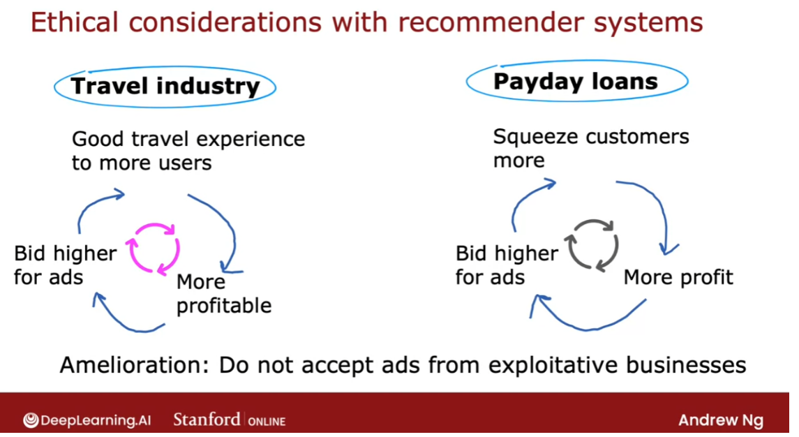
These are very
difficult problems that recommender
systems face. One amelioration might be to refuse to set ads from
exploitative businesses. Of course, that’s easy to say. But how do you define what is an exploitative business
and what is not, is a very difficult question. But as we build recommender systems for
advertising or for other things, I think these are
questions that each one of us working on
these technologies should ask ourselves so that we can hopefully invite open
discussion and debate, get multiple opinions
from multiple people, and try to come up with
design choices that allows our systems to try to do much more good than potential harm.

Let’s look at some
other examples. It’s been widely reported
in the news that maximizing user
engagement such as the amount of time that someone watches
videos on a website or the amount of time someone
spends on social media. This has led to
large social media and video sharing sites to amplify conspiracy theories
or hate and toxicity because conspiracy theories
and certain types of hate toxic content is highly engaging and causes people to
spend a lot of time on it.

Even if the effect of amplifying conspiracy
theories amplify hidden toxicity turns out to be harmful to individuals
and to society at large. One amelioration for this
partial and imperfect is to try to filter out problematic contents
such as hate speech, fraud, scams, maybe certain
types the violent content.

Again, the definitions of
what exactly we should filter out is surprisingly
tricky to develop. And this is a set of
problems that I think companies and individuals and even governments have to
continue to wrestle with.

Just one last example. When a user goes to
many apps or websites, I think users think
the app or website I tried to recommend to the user thinks that
they will like. I think many users don’t realize that many apps and
websites are trying to maximize their profit
rather than necessarily the user’s enjoyment of the media items that
are being recommended. I would encourage you and other companies if
at all possible, to be transparent
with users about a criteria by which you’re deciding what to
recommend to them. I know this isn’t always
easy, but ultimately, I hope that being more transparent with
users about why we’re showing them and why
will increase trust and also cause our systems to
do more good for society.

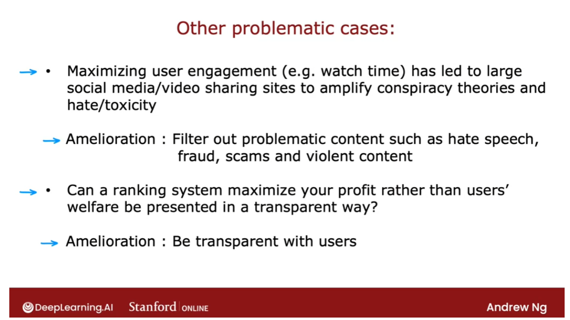
Recommender systems are
very powerful technology, a very profitable, a very
lucrative technology. There are also some
problematic use cases. If you are building one
of these systems using recommender technology or really any other machine
learning or other technology. I hope you think through not just the benefits
you can create, but also the possible harm and invite diverse perspectives
and discuss and debate. Please only build things
and do things that you really believe can
be society better off. I hope that collectively, all of us in AI can
only do work that makes people better off.

Thanks for listening. We have just one
more video to go in recommender systems in
which we take a look at some practical tips
for how to implement a content-based filtering
algorithm in TensorFlow. Let’s go on to that last
video on recommender systems.

TensorFlow implementation of content-based filtering

In the practice lab, you
see how to implement content-based filtering
in TensorFlow. What I’d like to
do in this video is just set through
of you a few of the key concepts in the code that you get to play
with. Let’s take a look. Recall that our code
has started with a user network as well
as a movie that’s work.

The way you can implement
this in TensorFlow is, it’s very similar to
how we have previously implemented a neural network
with a set of dense layers. We’re going to use
a sequential model. We then in this example have two dense layers with the number of hidden
units specified here, and the final layer has 32
units and output’s 32 numbers.

Then for the movie network, I’m going to call it
the item network, because the movies
are the items here, this is what the
code looks like. Once again, we have coupled
dense hidden layers, followed by this layer, which outputs 32 numbers. For the hidden layers, we’ll use our default choice of
activation function, which is the relu
activation function. Next, we need to tell TensorFlow Keras how to feed the user features
or the item features, that is the movie features
to the two neural networks. This is the syntax for doing so.

That extracts out the
input features for the user and then
feeds it to the user and that we had defined
up here to compute vu, the vector for the user. Then one additional step
that turns out to make this algorithm work a bit
better is at this line here, which normalizes the vector
vu to have length one. This normalizes the length, also called the l2 norm, but basically the length of the vector vu to
be equal to one. Then we do the same thing
for the item network, for the movie network. This extract out the item
features and feeds it to the item neural network
that we defined up there This computes the
movie vector vm. Then finally, the step also normalizes that vector
to have length one.

After having computed vu and vm, we then have to take the dot product between
these two vectors. This is the syntax for doing so. Keras has a special layer type, notice we had here tf
keras layers dense, here this is tf
keras layers dot. It turns out that there’s
a special Keras layer, they just takes a dot
product between two numbers. We’re going to use that to take the dot product between
the vectors vu and vm. This gives the output
of the neural network. This gives the final prediction.

Finally, to tell keras what are the inputs and
outputs of the model, this line tells it that the overall model is
a model with inputs being the user features and the movie or the item
features and the output, this is output that we
just defined up above.

The cost function that we’ll
use to train this model is going to be the mean
squared error cost function. These are the key
code snippets for implementing content-based
filtering as a neural network. You see the rest of the code in the practice lab but hopefully you’ll be
able to play with that and see how all these
code snippets fit together into working TensorFlow
implementation of a content-based
filtering algorithm.

It turns out that there’s one other step that I didn’t
talk about previously, but if you do this, which is normalize the
length of the vector vu, that makes the algorithm
work a bit better. TensorFlows has this
l2 normalized motion that normalizes the vector, is also called normalizing
the l2 norm of the vector, hence the name of the function.

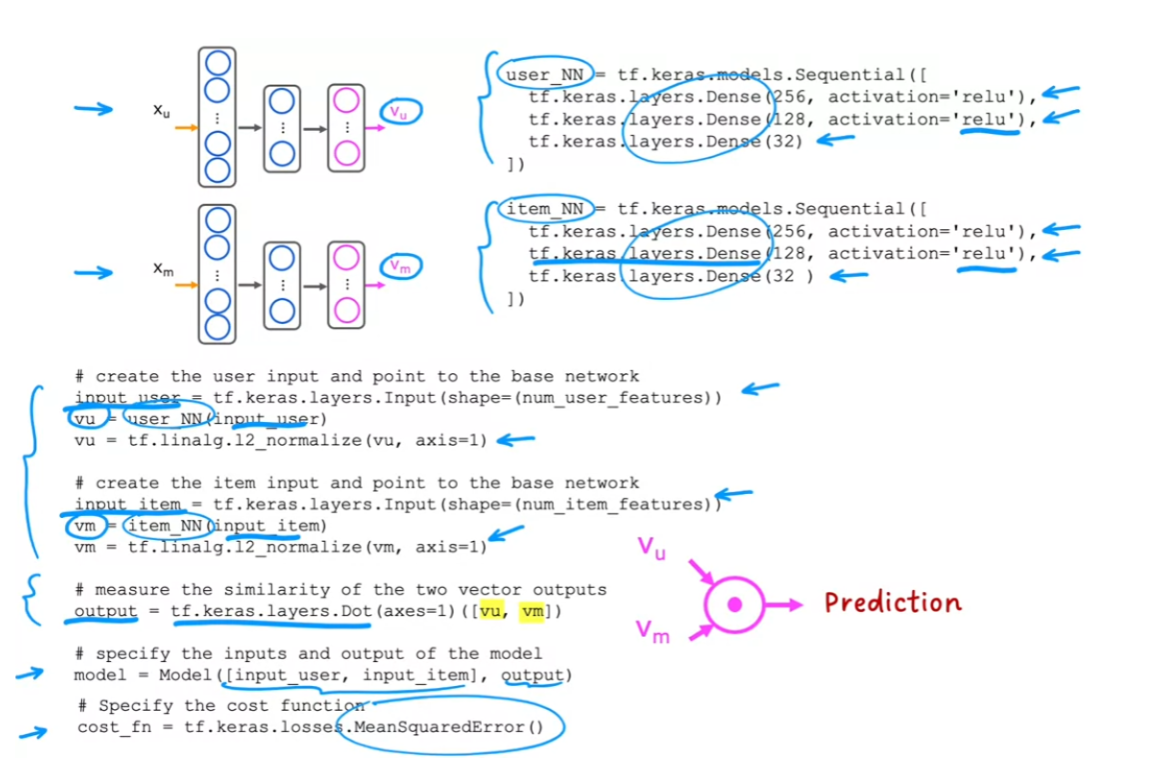
That’s it. Thanks for
sticking with me through all this material on
recommender systems, it is an exciting technology. I hope you enjoy playing with these ideas and codes in the
practice labs for this week. That takes us to the lots of these videos on
recommender systems and to the end of the next to final week for this
specialization. I look forward to seeing
you next week as well. We’ll talk about the
exciting technology of reinforcement learning. Hope you have fun with
the quizzes and with the practice labs and I look forward to
seeing you next week.

[7] Practice Quiz: Content-based filtering

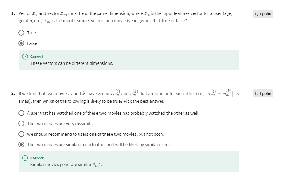
第三题是多选题，每个选项都是一幅图

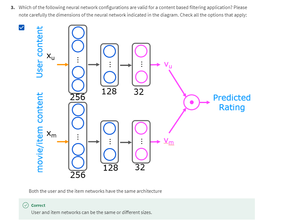
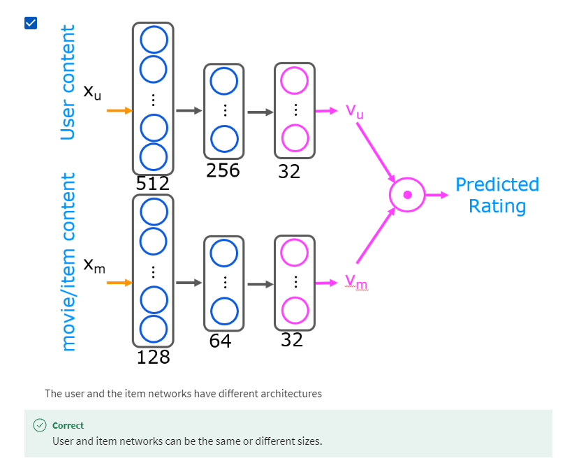
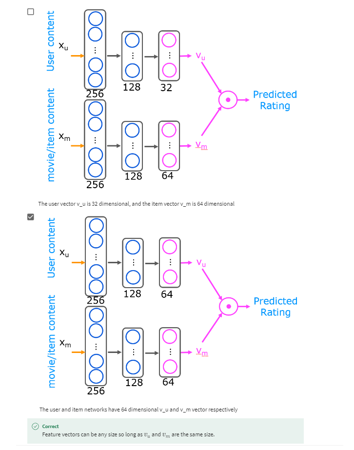
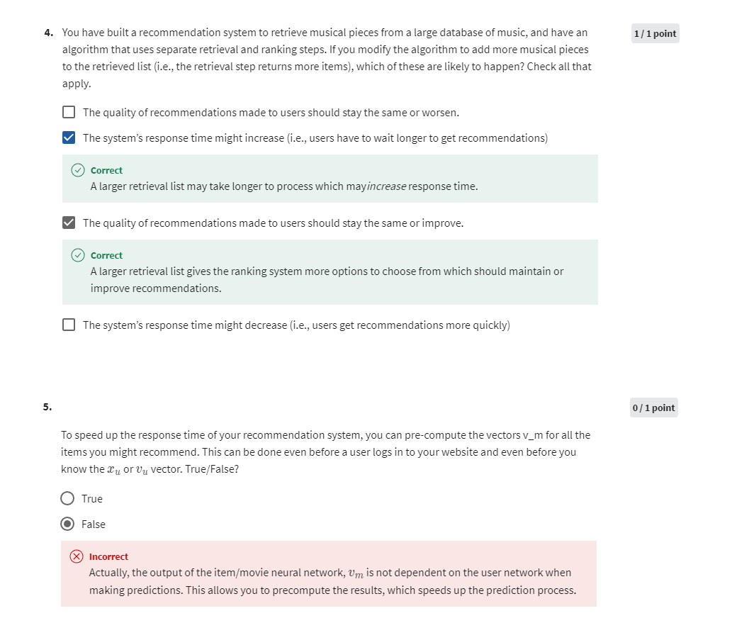
[8] Practice lab 2

In this lab, you will implement a content-based collaborative filtering recommender system for movies. This lab will use neural networks to generate the user and movie vectors.

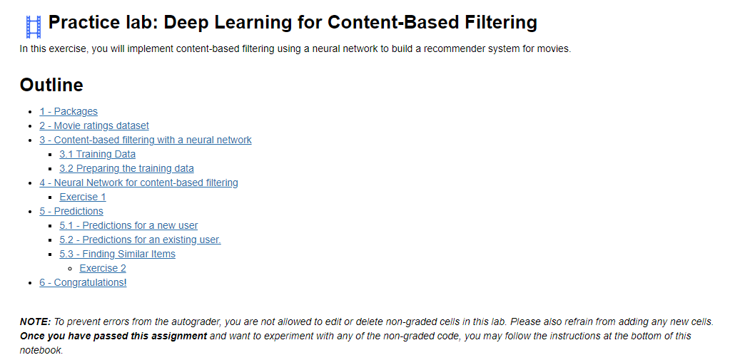
1 - Packages

We will use familiar packages, NumPy, TensorFlow and helpful routines from scikit-learn. We will also use tabulate to neatly print tables and Pandas to organize tabular data.

import numpy as np
import numpy.ma as ma
import pandas as pd
import tensorflow as tf
from tensorflow import keras
from sklearn.preprocessing import StandardScaler, MinMaxScaler
from sklearn.model_selection import train_test_split
import tabulate
from recsysNN_utils import *
pd.set_option("display.precision", 1)

2 - Movie ratings dataset

The data set is derived from the MovieLens ml-latest-small dataset.

[F. Maxwell Harper and Joseph A. Konstan. 2015. The MovieLens Datasets: History and Context. ACM Transactions on Interactive Intelligent Systems (TiiS) 5, 4: 19:1–19:19. https://doi.org/10.1145/2827872]

The original dataset has roughly 9000 movies rated by 600 users with ratings on a scale of 0.5 to 5 in 0.5 step increments. The dataset has been reduced in size to focus on movies from the years since 2000 and popular genres. The reduced dataset has $n_u=397$ users, $n_m=847$ movies and 25521 ratings. For each movie, the dataset provides a movie title, release date, and one or more genres. For example “Toy Story 3” was released in 2010 and has several genres: “Adventure|Animation|Children|Comedy|Fantasy”. This dataset contains little information about users other than their ratings. This dataset is used to create training vectors for the neural networks described below.
Let’s learn a bit more about this data set. The table below shows the top 10 movies ranked by the number of ratings. These movies also happen to have high average ratings. How many of these movies have you watched?

top10_df = pd.read_csv("./data/content_top10_df.csv")
bygenre_df = pd.read_csv("./data/content_bygenre_df.csv")
top10_df

Output

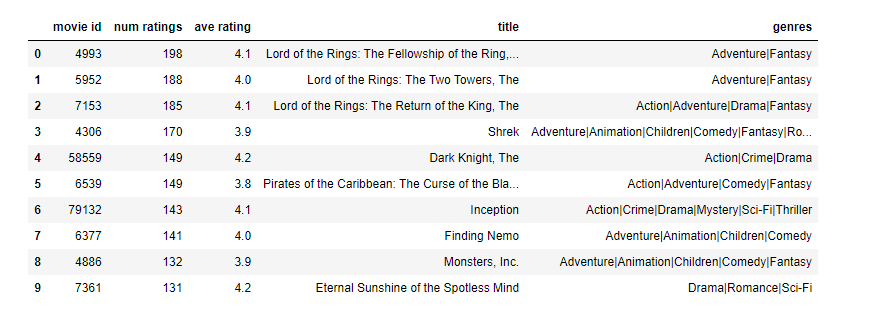
The next table shows information sorted by genre. The number of ratings per genre vary substantially. Note that a movie may have multiple genre’s so the sum of the ratings below is larger than the number of original ratings.

bygenre_df

Output

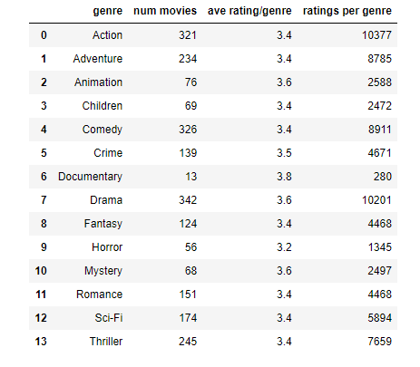
3 - Content-based filtering with a neural network

In the collaborative filtering lab, you generated two vectors, a user vector and an item/movie vector whose dot product would predict a rating. The vectors were derived solely from the ratings.

Content-based filtering also generates a user and movie feature vector but recognizes there may be other information available about the user and/or movie that may improve the prediction. The additional information is provided to a neural network which then generates the user and movie vector as shown below.

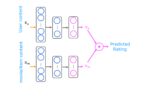
3.1 Training Data

The movie content provided to the network is a combination of the original data and some ‘engineered features’. Recall the feature engineering discussion and lab from Course 1, Week 2, lab 4. The original features are the year the movie was released and the movie’s genre’s presented as a one-hot vector. There are 14 genres. The engineered feature is an average rating derived from the user ratings.

The user content is composed of engineered features. A per genre average rating is computed per user. Additionally, a user id, rating count and rating average are available but not included in the training or prediction content. They are carried with the data set because they are useful in interpreting data.

The training set consists of all the ratings made by the users in the data set. Some ratings are repeated to boost the number of training examples of underrepresented genre’s. The training set is split into two arrays with the same number of entries, a user array and a movie/item array.

Below, let’s load and display some of the data.

# Load Data, set configuration variables
item_train, user_train, y_train, item_features, user_features, item_vecs, movie_dict, user_to_genre = load_data()num_user_features = user_train.shape[1] - 3  # remove userid, rating count and ave rating during training
num_item_features = item_train.shape[1] - 1  # remove movie id at train time
uvs = 3  # user genre vector start
ivs = 3  # item genre vector start
u_s = 3  # start of columns to use in training, user
i_s = 1  # start of columns to use in training, items
print(f"Number of training vectors: {len(item_train)}")

Output

Number of training vectors: 50884

Let’s look at the first few entries in the user training array.

pprint_train(user_train, user_features, uvs,  u_s, maxcount=5)

Output

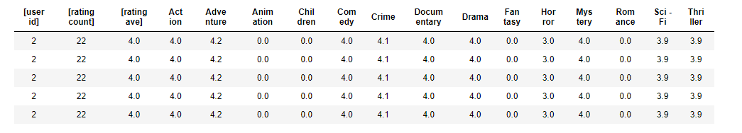
Some of the user and item/movie features are not used in training. In the table above, the features in brackets “[]” such as the “user id”, “rating count” and “rating ave” are not included when the model is trained and used.
Above you can see the per genre rating average for user 2. Zero entries are genre’s which the user had not rated. The user vector is the same for all the movies rated by a user.
Let’s look at the first few entries of the movie/item array.

pprint_train(item_train, item_features, ivs, i_s, maxcount=5, user=False)

Output

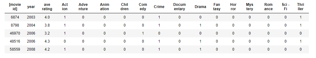
Above, the movie array contains the year the film was released, the average rating and an indicator for each potential genre. The indicator is one for each genre that applies to the movie. The movie id is not used in training but is useful when interpreting the data.

print(f"y_train[:5]: {y_train[:5]}")

Output

y_train[:5]: [4.  3.5 4.  4.  4.5]

The target, y, is the movie rating given by the user.

Above, we can see that movie 6874 is an Action/Crime/Thriller movie released in 2003. User 2 rates action movies as 3.9 on average. MovieLens users gave the movie an average rating of 4. ‘y’ is 4 indicating user 2 rated movie 6874 as a 4 as well. A single training example consists of a row from both the user and item arrays and a rating from y_train.

3.2 Preparing the training data

Recall in Course 1, Week 2, you explored feature scaling as a means of improving convergence. We’ll scale the input features using the scikit learn StandardScaler. This was used in Course 1, Week 2, Lab 5. Below, the inverse_transform is also shown to produce the original inputs. We’ll scale the target ratings using a Min Max Scaler which scales the target to be between -1 and 1. scikit learn MinMaxScaler

# scale training data
item_train_unscaled = item_train
user_train_unscaled = user_train
y_train_unscaled    = y_trainscalerItem = StandardScaler()
scalerItem.fit(item_train)
item_train = scalerItem.transform(item_train)scalerUser = StandardScaler()
scalerUser.fit(user_train)
user_train = scalerUser.transform(user_train)scalerTarget = MinMaxScaler((-1, 1))
scalerTarget.fit(y_train.reshape(-1, 1))
y_train = scalerTarget.transform(y_train.reshape(-1, 1))
#ynorm_test = scalerTarget.transform(y_test.reshape(-1, 1))print(np.allclose(item_train_unscaled, scalerItem.inverse_transform(item_train)))
print(np.allclose(user_train_unscaled, scalerUser.inverse_transform(user_train)))

这段代码中使用了 StandardScaler 和 MinMaxScaler 这两种数据标准化（或称为归一化）的方法。这些方法主要用于将数据转换为具有特定均值和标准差（或最小值和最大值）的分布，以便更好地训练机器学习模型。

1. StandardScaler：

   • StandardScaler 是一种常见的数据标准化方法，它通过减去均值并除以标准差的方式将数据进行标准化，使得标准化后的数据具有均值为0，标准差为1的标准正态分布。
   • 使用 fit() 方法可以计算训练集的均值和标准差，并使用 transform() 方法对数据进行标准化。
   • 在这段代码中，先使用 fit() 方法计算训练集 item_train 和 user_train 的均值和标准差，然后分别使用 transform() 方法对它们进行标准化。这样做的目的是将这两个特征的数据缩放到均值为0，标准差为1的范围内。

2. MinMaxScaler：

   • MinMaxScaler 是一种将数据缩放到指定范围内的方法，通常是 [0, 1] 或 [-1, 1]。
   • 使用 fit() 方法可以计算训练集的最大值和最小值，并使用 transform() 方法对数据进行缩放。
   • 在这段代码中，先使用 fit() 方法计算训练集 y_train 的最大值和最小值，然后使用 transform() 方法将其缩放到指定的范围内。这样做的目的是使目标变量的数据落在指定的范围内，以便更好地训练模型。

综上所述，StandardScaler 和 MinMaxScaler 都是常用的数据预处理工具，用于将特征数据标准化或缩放到合适的范围内，以提高模型的训练效果。

Output

True

True

To allow us to evaluate the results, we will split the data into training and test sets as was discussed in Course 2, Week 3. Here we will use sklean train_test_split to split and shuffle the data. Note that setting the initial random state to the same value ensures item, user, and y are shuffled identically.

item_train, item_test = train_test_split(item_train, train_size=0.80, shuffle=True, random_state=1)
user_train, user_test = train_test_split(user_train, train_size=0.80, shuffle=True, random_state=1)
y_train, y_test       = train_test_split(y_train,    train_size=0.80, shuffle=True, random_state=1)
print(f"movie/item training data shape: {item_train.shape}")
print(f"movie/item test data shape: {item_test.shape}")

Output

movie/item training data shape: (40707, 17)
movie/item test data shape: (10177, 17)

The scaled, shuffled data now has a mean of zero.

pprint_train(user_train, user_features, uvs, u_s, maxcount=5)

Output

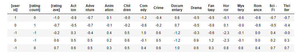
4 - Neural Network for content-based filtering

Now, let’s construct a neural network as described in the figure above. It will have two networks that are combined by a dot product. You will construct the two networks. In this example, they will be identical. Note that these networks do not need to be the same. If the user content was substantially larger than the movie content, you might elect to increase the complexity of the user network relative to the movie network. In this case, the content is similar, so the networks are the same.

Exercise 1

• Use a Keras sequential model
  • The first layer is a dense layer with 256 units and a relu activation.
  • The second layer is a dense layer with 128 units and a relu activation.
  • The third layer is a dense layer with num_outputs units and a linear or no activation.

The remainder of the network will be provided. The provided code does not use the Keras sequential model but instead uses the Keras functional api. This format allows for more flexibility in how components are interconnected.

# GRADED_CELL
# UNQ_C1num_outputs = 32
tf.random.set_seed(1)
user_NN = tf.keras.models.Sequential([### START CODE HERE ###     tf.keras.layers.Dense(256, activation="relu"),tf.keras.layers.Dense(128, activation="relu"),tf.keras.layers.Dense(num_outputs)### END CODE HERE ###  
])item_NN = tf.keras.models.Sequential([### START CODE HERE ###     tf.keras.layers.Dense(256, activation="relu"),tf.keras.layers.Dense(128, activation="relu"),tf.keras.layers.Dense(num_outputs)### END CODE HERE ###  
])# create the user input and point to the base network
input_user = tf.keras.layers.Input(shape=(num_user_features))
vu = user_NN(input_user)
vu = tf.linalg.l2_normalize(vu, axis=1)# create the item input and point to the base network
input_item = tf.keras.layers.Input(shape=(num_item_features))
vm = item_NN(input_item)
vm = tf.linalg.l2_normalize(vm, axis=1)# compute the dot product of the two vectors vu and vm
output = tf.keras.layers.Dot(axes=1)([vu, vm])# specify the inputs and output of the model
model = tf.keras.Model([input_user, input_item], output)model.summary()

Output

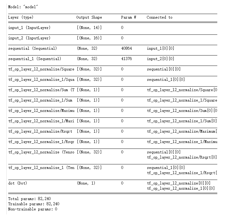
Test

# Public tests
from public_tests import *
test_tower(user_NN)
test_tower(item_NN)

Output

All tests passed!
All tests passed!

We will use a mean squared error loss and an Adam optimizer.

tf.random.set_seed(1)
cost_fn = tf.keras.losses.MeanSquaredError()
opt = keras.optimizers.Adam(learning_rate=0.01)
model.compile(optimizer=opt,loss=cost_fn)

tf.random.set_seed(1)
model.fit([user_train[:, u_s:], item_train[:, i_s:]], y_train, epochs=30)

Output

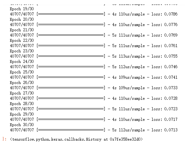
Evaluate the model to determine loss on the test data.

model.evaluate([user_test[:, u_s:], item_test[:, i_s:]], y_test)

Output

0.08146006993124337

It is comparable to the training loss indicating the model has not substantially overfit the training data.

5 - Predictions

Below, you’ll use your model to make predictions in a number of circumstances.

5.1 - Predictions for a new user

First, we’ll create a new user and have the model suggest movies for that user. After you have tried this on the example user content, feel free to change the user content to match your own preferences and see what the model suggests. Note that ratings are between 0.5 and 5.0, inclusive, in half-step increments.

new_user_id = 5000
new_rating_ave = 0.0
new_action = 0.0
new_adventure = 5.0
new_animation = 0.0
new_childrens = 0.0
new_comedy = 0.0
new_crime = 0.0
new_documentary = 0.0
new_drama = 0.0
new_fantasy = 5.0
new_horror = 0.0
new_mystery = 0.0
new_romance = 0.0
new_scifi = 0.0
new_thriller = 0.0
new_rating_count = 3user_vec = np.array([[new_user_id, new_rating_count, new_rating_ave,new_action, new_adventure, new_animation, new_childrens,new_comedy, new_crime, new_documentary,new_drama, new_fantasy, new_horror, new_mystery,new_romance, new_scifi, new_thriller]])

The new user enjoys movies from the adventure, fantasy genres. Let’s find the top-rated movies for the new user.
Below, we’ll use a set of movie/item vectors, item_vecs that have a vector for each movie in the training/test set. This is matched with the new user vector above and the scaled vectors are used to predict ratings for all the movies.

# generate and replicate the user vector to match the number movies in the data set.
user_vecs = gen_user_vecs(user_vec,len(item_vecs))# scale our user and item vectors
suser_vecs = scalerUser.transform(user_vecs)
sitem_vecs = scalerItem.transform(item_vecs)# make a prediction
y_p = model.predict([suser_vecs[:, u_s:], sitem_vecs[:, i_s:]])# unscale y prediction 
y_pu = scalerTarget.inverse_transform(y_p)# sort the results, highest prediction first
sorted_index = np.argsort(-y_pu,axis=0).reshape(-1).tolist()  #negate to get largest rating first
sorted_ypu   = y_pu[sorted_index]
sorted_items = item_vecs[sorted_index]  #using unscaled vectors for displayprint_pred_movies(sorted_ypu, sorted_items, movie_dict, maxcount = 10)

Output

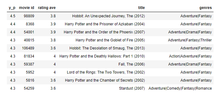
5.2 - Predictions for an existing user.

Let’s look at the predictions for “user 2”, one of the users in the data set. We can compare the predicted ratings with the model’s ratings.

uid = 2 
# form a set of user vectors. This is the same vector, transformed and repeated.
user_vecs, y_vecs = get_user_vecs(uid, user_train_unscaled, item_vecs, user_to_genre)# scale our user and item vectors
suser_vecs = scalerUser.transform(user_vecs)
sitem_vecs = scalerItem.transform(item_vecs)# make a prediction
y_p = model.predict([suser_vecs[:, u_s:], sitem_vecs[:, i_s:]])# unscale y prediction 
y_pu = scalerTarget.inverse_transform(y_p)# sort the results, highest prediction first
sorted_index = np.argsort(-y_pu,axis=0).reshape(-1).tolist()  #negate to get largest rating first
sorted_ypu   = y_pu[sorted_index]
sorted_items = item_vecs[sorted_index]  #using unscaled vectors for display
sorted_user  = user_vecs[sorted_index]
sorted_y     = y_vecs[sorted_index]#print sorted predictions for movies rated by the user
print_existing_user(sorted_ypu, sorted_y.reshape(-1,1), sorted_user, sorted_items, ivs, uvs, movie_dict, maxcount = 50)

Output

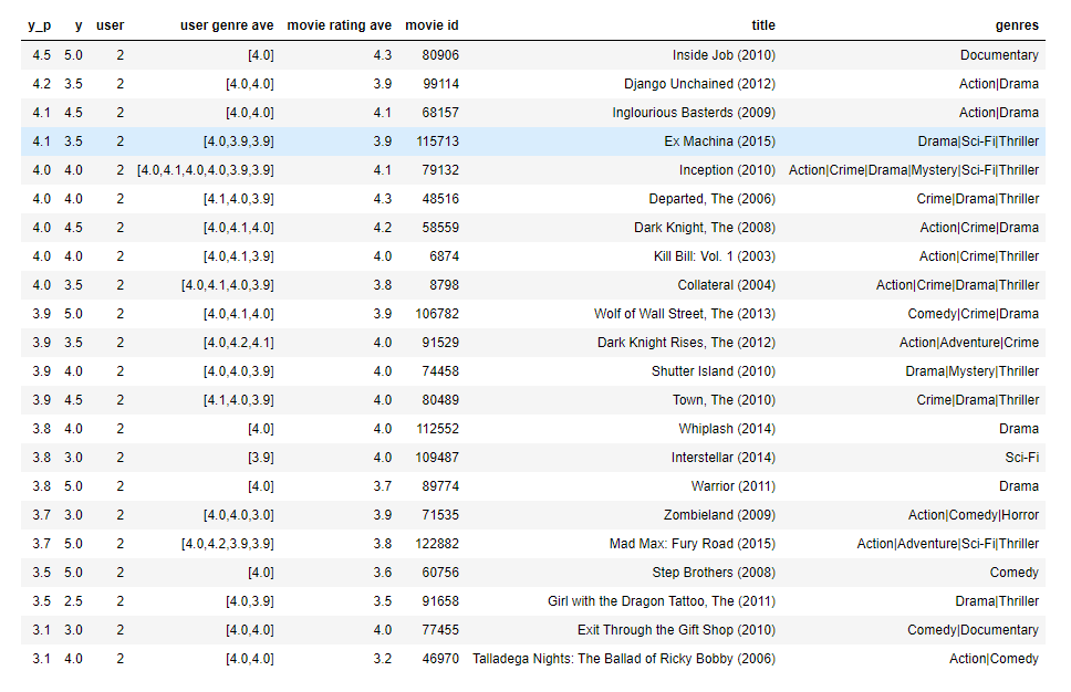
The model prediction is generally within 1 of the actual rating though it is not a very accurate predictor of how a user rates specific movies. This is especially true if the user rating is significantly different than the user’s genre average. You can vary the user id above to try different users. Not all user id’s were used in the training set.

5.3 - Finding Similar Items

The neural network above produces two feature vectors, a user feature vector $v_u$, and a movie feature vector, $v_m$. These are 32 entry vectors whose values are difficult to interpret. However, similar items will have similar vectors. This information can be used to make recommendations. For example, if a user has rated “Toy Story 3” highly, one could recommend similar movies by selecting movies with similar movie feature vectors.

A similarity measure is the squared distance between the two vectors $ \mathbf{v_m^{(k)}}$ and ${\mathbf{v}}_{\mathbf{m}}^{(\mathbf{i})}$ :
$${\Vert {\mathbf{v}}_{\mathbf{m}}^{(\mathbf{k})}-{\mathbf{v}}_{\mathbf{m}}^{(\mathbf{i})}\Vert }^2=\sum _{l=1}^n(v_{m_l}^{(k)}-v_{m_l}^{(i)}{)}^2\text{\hspace{1em}(1)}$$

Exercise 2

Write a function to compute the square distance.

# GRADED_FUNCTION: sq_dist
# UNQ_C2
def sq_dist(a,b):"""Returns the squared distance between two vectorsArgs:a (ndarray (n,)): vector with n featuresb (ndarray (n,)): vector with n featuresReturns:d (float) : distance"""### START CODE HERE ###     d = np.sum(np.square(a - b))### END CODE HERE ###     return d

a1 = np.array([1.0, 2.0, 3.0]); b1 = np.array([1.0, 2.0, 3.0])
a2 = np.array([1.1, 2.1, 3.1]); b2 = np.array([1.0, 2.0, 3.0])
a3 = np.array([0, 1, 0]);       b3 = np.array([1, 0, 0])
print(f"squared distance between a1 and b1: {sq_dist(a1, b1):0.3f}")
print(f"squared distance between a2 and b2: {sq_dist(a2, b2):0.3f}")
print(f"squared distance between a3 and b3: {sq_dist(a3, b3):0.3f}")

Output

squared distance between a1 and b1: 0.000
squared distance between a2 and b2: 0.030
squared distance between a3 and b3: 2.000

Expected Output:

squared distance between a1 and b1: 0.000
squared distance between a2 and b2: 0.030
squared distance between a3 and b3: 2.000

# Public tests
test_sq_dist(sq_dist)

Output

All tests passed!

A matrix of distances between movies can be computed once when the model is trained and then reused for new recommendations without retraining. The first step, once a model is trained, is to obtain the movie feature vector, $v_m$, for each of the movies. To do this, we will use the trained item_NN and build a small model to allow us to run the movie vectors through it to generate $v_m$.

input_item_m = tf.keras.layers.Input(shape=(num_item_features))    # input layer
vm_m = item_NN(input_item_m)                                       # use the trained item_NN
vm_m = tf.linalg.l2_normalize(vm_m, axis=1)                        # incorporate normalization as was done in the original model
model_m = tf.keras.Model(input_item_m, vm_m)                                
model_m.summary()

Output

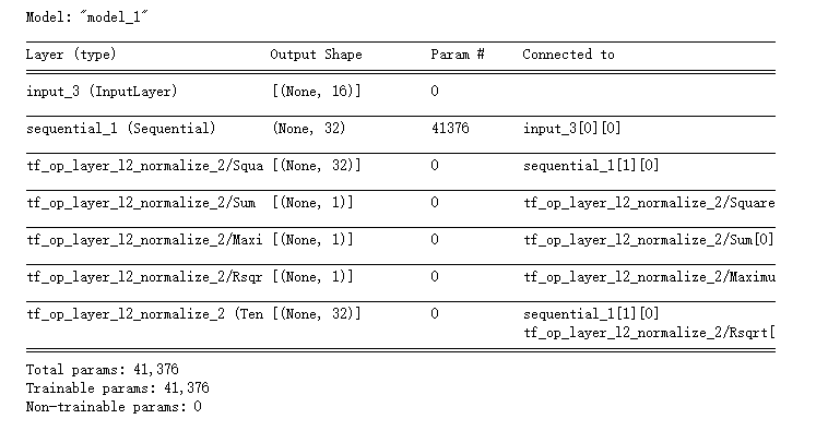
第一行代码是使用 TensorFlow 的 Keras API 创建了一个输入层（input layer），用于接收项目特征的输入数据。让我解释一下其中的参数：

• tf.keras.layers.Input：这是 Keras 中的一个函数，用于创建一个输入层。
• shape=(num_item_features)：这个参数指定了输入数据的形状，即项目特征的数量。num_item_features 表示项目特征的数量。这个参数告诉模型输入层应该期望接收的数据形状。

综合起来，这行代码创建了一个用于接收项目特征数据的输入层，该输入层的数据形状是 (num_item_features,)，其中 num_item_features 是项目特征的数量。在神经网络中，输入层用于接收原始数据，并将其传递给网络的下一层进行处理。

Once you have a movie model, you can create a set of movie feature vectors by using the model to predict using a set of item/movie vectors as input. item_vecs is a set of all of the movie vectors. It must be scaled to use with the trained model. The result of the prediction is a 32 entry feature vector for each movie.

scaled_item_vecs = scalerItem.transform(item_vecs)
vms = model_m.predict(scaled_item_vecs[:,i_s:])
print(f"size of all predicted movie feature vectors: {vms.shape}")

Output

size of all predicted movie feature vectors: (847, 32)

Let’s now compute a matrix of the squared distance between each movie feature vector and all other movie feature vectors:

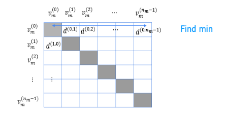
We can then find the closest movie by finding the minimum along each row. We will make use of numpy masked arrays to avoid selecting the same movie. The masked values along the diagonal won’t be included in the computation.

count = 50  # number of movies to display
dim = len(vms)
dist = np.zeros((dim,dim))for i in range(dim):for j in range(dim):dist[i,j] = sq_dist(vms[i, :], vms[j, :])m_dist = ma.masked_array(dist, mask=np.identity(dist.shape[0]))  # mask the diagonaldisp = [["movie1", "genres", "movie2", "genres"]]
for i in range(count):min_idx = np.argmin(m_dist[i])movie1_id = int(item_vecs[i,0])movie2_id = int(item_vecs[min_idx,0])disp.append( [movie_dict[movie1_id]['title'], movie_dict[movie1_id]['genres'],movie_dict[movie2_id]['title'], movie_dict[movie1_id]['genres']])
table = tabulate.tabulate(disp, tablefmt='html', headers="firstrow")
table

Output部分输出

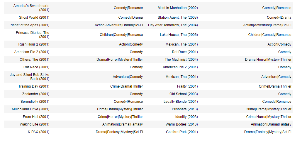
The results show the model will generally suggest a movie with similar genre’s.

6 - Congratulations!

You have completed a content-based recommender system.

This structure is the basis of many commercial recommender systems. The user content can be greatly expanded to incorporate more information about the user if it is available. Items are not limited to movies. This can be used to recommend any item, books, cars or items that are similar to an item in your ‘shopping cart’.

Grades

[9] Principal Component Analysis

Reducing the number of features (optional)

I hope you enjoyed
the videos on how you can build your own
recommender system. Before we wrap up
this week in this and a few other optional videos
I’d like to share with you an unsupervised
learning algorithm called principal
components analysis.

This is an algorithm that is commonly used for visualization. Specifically, if you have a dataset with
a lot of features, say 10 features or 50 features or even
thousands of features, you can’t plot 1,000
dimensional data. PCA, or principal
components analysis is an algorithm that lets you take data with a lot
of features, 50, 1,000, even more, and reduce the number of features
to two features, maybe three features,
so that you can plot it and visualize it. Is commonly used by data scientists to
visualize the data, to figure out what
might be going on.

Let’s take a look at how PCA, principal components
analysis works. To describe PCA, I’m going
to use as a running example, if you have data from a
collection of passenger cars, and passenger cars can
have a lot of features. You may know the length of the car or the width of the car, maybe the diameter of the wheel, or maybe the height of the car, and many other features of cars. If you want to reduce the number of features
so you can visualize it, how can you use PCA to do so?

For the first example, let’s say you’re given a
dataset with two features. The feature x_1 is the
length of the car, like so, and the
second feature x_2, is the width of the car, which is measured like so. It turns out that
in most countries, because of constraints
about the width of the road the cars drive on, width of the car
which has got to fit within the width of the
road of a single lane, tends not to vary that much. For example, in
the United States, most cars are, let’s call it about
1.8 meters wide, that’s just under six feet.

If you were to have
a collection of cars and the dataset of the length and
width of the cars, you will find that the
dataset might look like this, where x_1 varies quite a bit
because some cars are really long and x_2 varies
relatively little. If you want to reduce the
number of features, well, one thing you could do is
let us take x_1 because x_2 varies relatively
little from car to car.

It turns out that
PCA is an algorithm that when applied to
this data set will more or less automatically
decide to just take x_1, but it can do much
more than that.

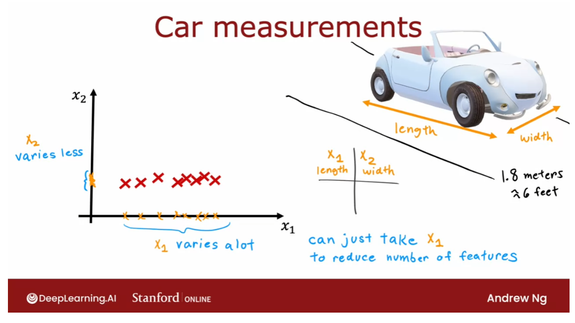
Let’s look at a second example where here x_1 is again
the length of the car, and let’s say that
in this dataset, x_2 is the diameter
of the wheel. The diameter of the wheel
does vary a little bit. If you were to plot the data, it might look like this. But again, if you want to simplify this dataset
to just one feature, you might decide, let’s
just take x_1 and forget x_2 and PCA when
applied to this dataset. Well, again, more or less, cause you to just
check the feature x_1. In both the examples we saw, only one of the two
features seemed to have a meaningful
degree of variation.

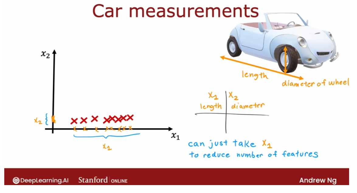
Here’s a more complex example. Say the feature x_1 is
the length of the car, so that varies quite a bit, and the feature x_2 here
is the height of the car, which also varies quite a bit. Some cars are much
taller than other cars. If you were to plot the data, you might get a dataset
that looks like this, where some cars are bigger and they tend to be
longer and taller, and some cars are a
little bit smaller. They tend to be not as
long and not as tall.

If you wanted to
reduce the number of features, what should you pick? You don’t want to pick
just x_1, the length, and ignore x_2 the height and you also don’t
want to pick just x_2, the height, and ignore
x_1, the length. It seems as if both x_1 and
x_2 have useful information. In this graph, x_1 and x_2 are the
two axes of this plot. Instead of being
limited to taking either the x_1 axis
or the x_2 axis, what if we had a third axis. I’m going to call this
new axis the z-axis.

To be clear, this is not
sticking out of this diagram. This is a combination
of x_1 and x_2. This is not a z-axis that’s sticking out in
the third dimension. This z-axis lies flat
within this plot. But why do we have
the z-axis which corresponds to something
about the size of the car? Given a car like this one
over here, its coordinate, meaning the value
on the x-axis tells us the length of the car
and the coordinate is just, what is this distance? Similarly its
coordinate, meaning, what is this distance on the x_2 axis tells us what
is the height of the car.

If we’re now going to
use the z-axis instead as one feature to capture what we know about this car
then is coordinate on the z-axis, meaning
this distance. That tells us roughly what
is the size of the car. We’ll formalize this in
the next few videos.

But the idea of PCA is to
find one or more new axes, such as z so that when you measure your datas
coordinates on the new axis, you end up still with very useful information
about the car. But maybe now,
instead of needing two numbers corresponding to the coordinates on
X_1 and X_2 axes, the length and height. You now need a few
numbers, in this case, only one number instead of two, to capture roughly
the size of the car.

In the example,
we’ve used so far, we were trying to reduce
the data from two numbers, X_1 and X_2 down to one number, the coordinate on the z-axis. In practice, PCA
is usually used to reduce a very large
number of features, say 10, 20, 50, even thousands of features, down to maybe two or three
features so that you can visualize the data in a two-dimensional or in a
three-dimensional plot.

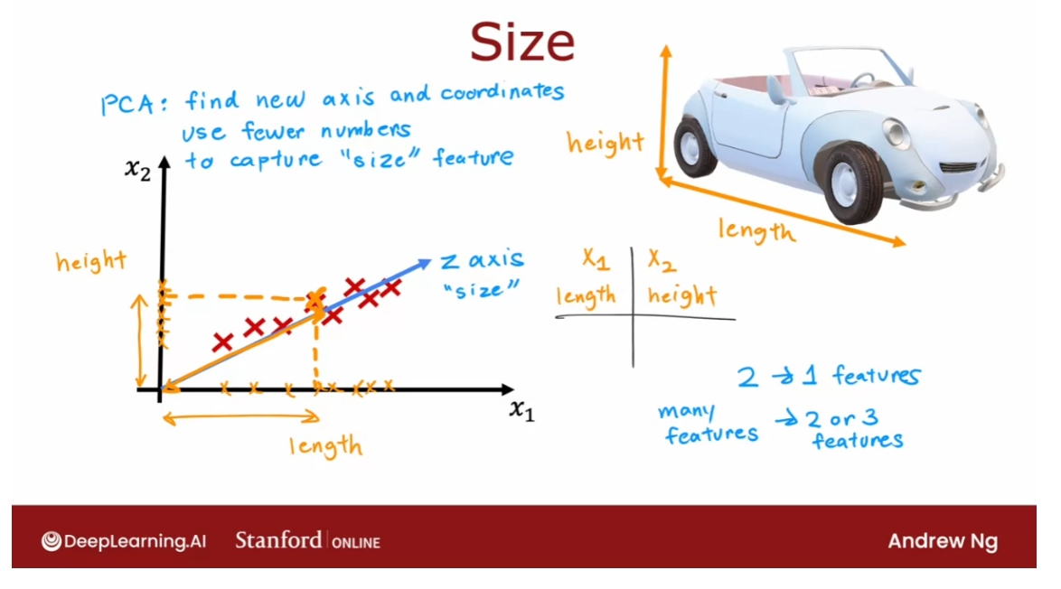
But for this video, because I could only draw on
a two-dimensional screen. I’m going to use mainly two or three-dimensional
data sets as my examples.

Let’s look at one more example. In this visualization, we
have a three-dimensional data set and notice that I can
rotate the data set here, so you can see it in 3D. But notice if I rotate
the data set like this, well, most of this data, even though it is in 3D, it actually lives on
a very thin surface. It’s almost as if
all the data lies on a two-dimensional pancake, even though the pancake lives in this
three-dimensional space.

A PCA, what you can do is, instead of having
three features, x_1, x_2, x_3, reduce it to two numbers, which we’re going to
call Z_1 and Z_2. When you do that, you can then visualize
the data on this Z_1, Z_2 axis and this becomes a convenient way to visualize
this data if you had to, say print on a piece of paper. I couldn’t dynamically rotate it like you’ll seeing
me do on the screen.

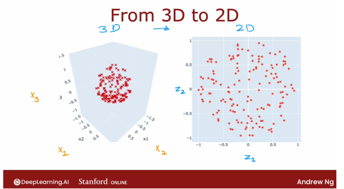
Here’s one more example. If you have data about the development status of
many different countries, you might have for example data about different countries, GDP, and that’s feature x_1. In addition, Let’s
say we also have the per capita GDP and also a measure of their Human
Development Index. The Human Development
Index was developed to measure the overall
progress of how well people in a country might be doing based on things
like the lifespan and education and so on or you might separately
have a feature corresponding to
the life expectancy in different countries
and so on and so forth.

If for each country
you have 50 features, how can you visualize this
data because you can’t plot 50 dimensional data on a two-dimensional
computer monitor. What PCAS will do is take these 50 features,
X_1,X_2,X_3,X_4, and so on and compress it down to two features
which I’m going to call Z_1 and Z_2 and you can then plot these different countries
values of z_1 and z_2.

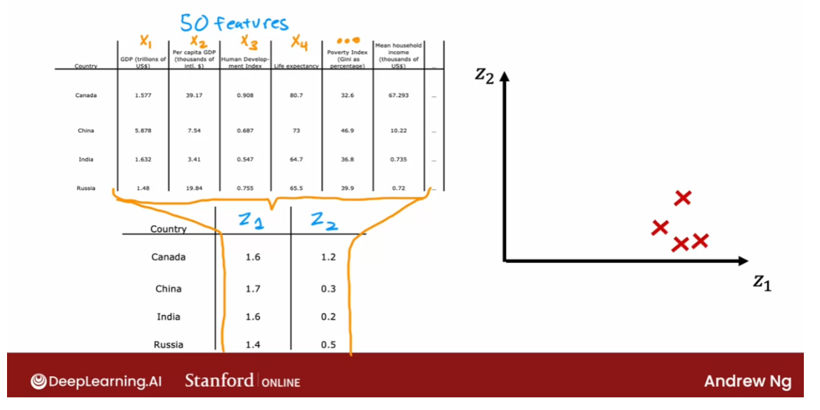
You might find for example
that Z_1 loosely corresponds to how big is the country
and what is this total GDP? Because larger countries
tend to have a higher GDP, because large countries
have many people, tend to have a larger economy and perhaps you find that Z_2 corresponds roughly
to the per person GDP or the amount of economic
activity per person.

For example, the United States, which is a relatively
large country and has relatively high per
person economic activity may be somewhere up here
to the up and right of this plot and a country
like Singapore, where I live many years as well, is a smaller country but it has relatively high per
person economic activity. Take on a lower value
on the z_1 axis, but still a relatively high
value on the z_2 axis.

Whereas a country like
this would be maybe a smaller country with lower per person
economic activity. Whereas the country like this
may be a large country with lower per person economic
activity and a figure like this lets you take a large number of
features, 50 features. Sometimes we also say
that’s 50 dimensional data. It just means we
have 50 features and reduce that to two features
or sometimes we say is two-dimensional data because
you can then plot it on this two-dimensional plot
like you’re seeing here.

Whenever I get a new data set, one of the things I’ll often
want to do is to visualize the data since that helps me understand what the
data looks like, what do the countries look like, or what do the cars seem
like in this data set or whatever data you
may be examining. You find also that
visualizing the data set will sometimes help you figure out something funny’s going
on in this datas. Something unexpected
is happening.

PCA is a powerful algorithm for taking data with
a lot of features, with a lot of dimensions
or high-dimensional data, and reducing it to two
or three features to two or three dimensional
data so you can plot it and visualize it and better understand what’s in your data. That’s what the PCA
algorithm can do for you. In the next video, let’s start to
take a look at how exactly the PCA algorithm works.

PCA algorithm (optional)

How does PCA work? If you have a dataset with
two features, x_1 and x_2. Initially, your
data is plotted or represented using
axes x_1 and x_2. But you want to replace these two features
with just one feature. How can you choose a new axis, let’s call it the z-axis, that is somehow a good
feature for capturing, of representing the data? Let’s take a look at
how PCA does this.

Here’s the data sets with
five training examples. Remember, this is an
unsupervised learning algorithm so we just have x_1 and x_2, there is no label y. An example here like this
may have coordinates x_1 equals 10 and x_2 equals 8. If we don’t want to
use the x_1, x_2 axes, how can we pick some
different axis with which to capture what’s in
the data or with which to represent the data?

One note on preprocessing, before applying the next few
steps of PCA the features should be first
normalized to have zero mean and I’ve
already done that here. If the features x_1 and x_2 take on very
different scales, for example, if you remember
our housing example, if x_1 was the size of
a house in square feet, and x_2 was the number
of bedrooms then x_1 could be 1,000 or
a couple of thousand, whereas x_2 is a small number. If the features take on
very different scales, then you will first
perform feature scaling before applying
the next few steps of PCA.

Assuming the features have been normalized to have zero mean, so subtract the mean from each feature and
then maybe apply feature scaling as well so the ranges are
not too far apart.

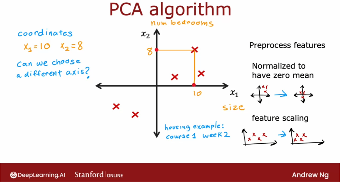
What does PCA do next? To examine what PCA does, let me remove the
x_1 and x_2 axes so that we’re just left with
the five training examples. This dot here
represents the origin. The position of zero
on this plot still. What we have to do
now with PCA is, pick one axis instead of the two axes that
we had previously with which to capture what’s important about
these five examples.

If we were to choose this
axis to be our new z-axis, it’s actually the
same as the x_1 axis just for this example. Then what we’re saying is
that for this example, we’re going to just
capture this value, this coordinate on the z-axis. For the second example, we’re going to
capture this value, and then this will
capture this value, and so on for all five examples. Another way of
saying this is that we’re going to take
each of these examples and project it down to
a point on the z-axis.

The word project refers to that you’re taking this example
and bringing it to the z-axis using
this line segment that’s at a 90-degree
angle to the z-axis. This little box here
is used to denote that this line segment is at
90 degrees to the z-axis. The term project
just means you’re taking a point and finding this corresponding
point on the z-axis using this line segment
that’s at 90 degrees.

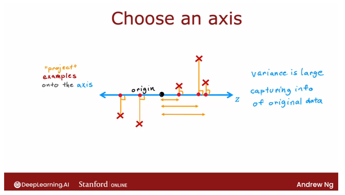
Picking this direction as a
z-axis is not a bad choice, but there’s some
even better choices. This choice isn’t
too bad because when you project your
examples onto the z-axis, you still capture quite a lot
of the spread of the data. These five points here, they’re pretty spread apart so you’re still
capturing a lot of the variation or a lot of the variance in the
original dataset. By that I mean these five
points are quite spread apart and so the variance or variation among
these five points, the projections of the data onto the z-axis is decently large. What that means is we’re
still capturing quite a lot of the information in the
original five examples.

Let’s look at some other
possible choices for the axis z. Here’s another choice. This is actually not a great choice. But if I were to choose
this as my z axis, then if I take those same five examples and project them
down to the z-axis, I end up with these five points. You notice that compare it
to the previous choice, these five points are
quite squished together. The amount they are
differing from each other, or their variance or the
variation is much less.

What this means is
with this choice of z, you’re capturing much less
of the information in the original dataset
because you’ve partially squish all
five examples together.

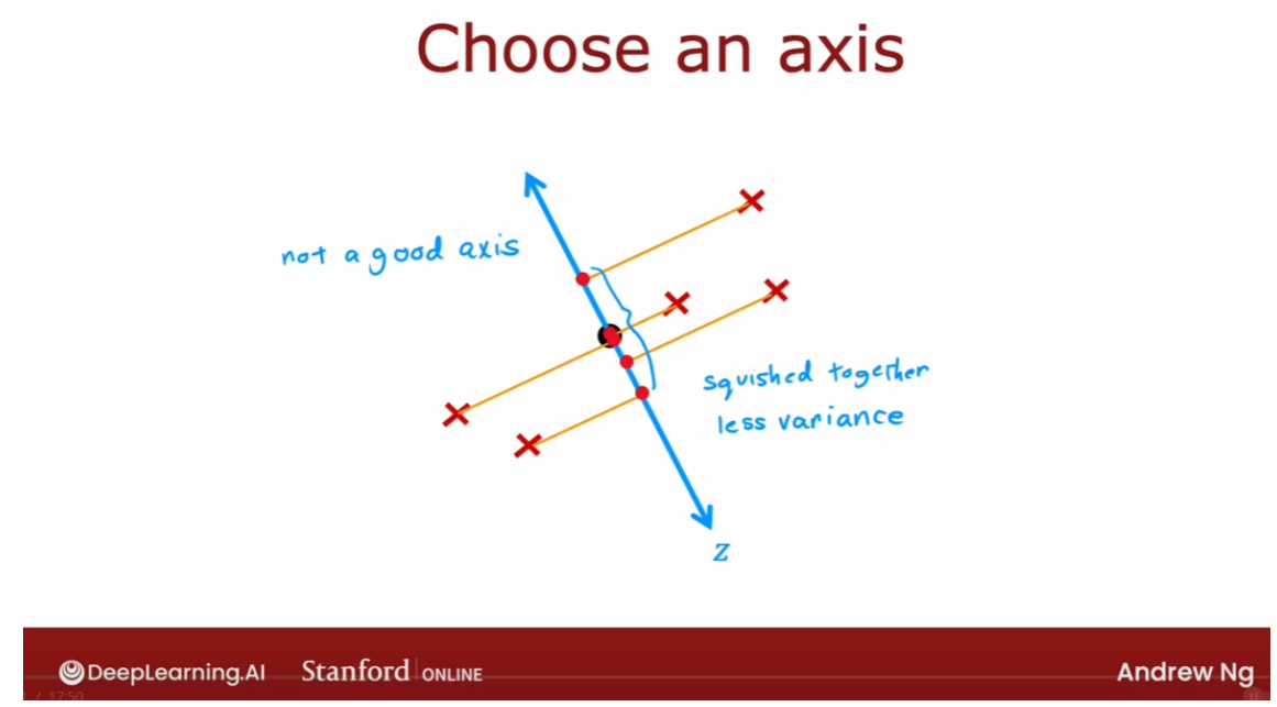
Let’s look at one last choice, which is if I choose
this to be the z-axis. This is actually a better choice than the previous
two that we saw, because if we take the data’s projections
onto the z-axis, we find that these
dots over here, they’re actually
quite far apart.

We’re capturing a lot
of the variation, a lot of the information
in the original dataset, even though we’re now using just one coordinate or one
number to represent or to capture each of the
training examples instead of two numbers or two
coordinates, X_1 and X_2.

In the PCA algorithm, this axis is called the
principal component. In the z-axis that when you
project the data onto it, you end up with the largest
possible amounts of variance. If you were to reduce the data to one axis or to one feature, this principal component
is actually a good choice, and this is what PCA will do. If you want to reduce the data to one-dimensional feature, then it will choose this
principal component.

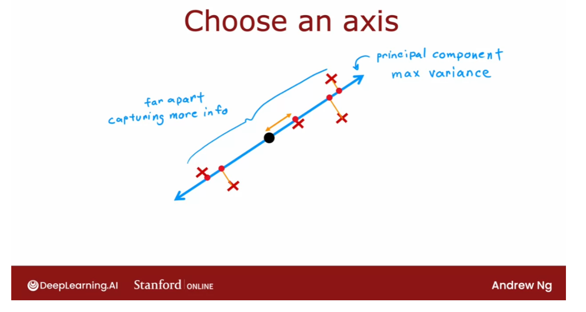
Let me show you a
visualization of how different choices of the
axis affects the projection. Here we have 10
training examples, and as we slide
this slider here, and you can play with this in one of the optional
labs yourself. As you slide the slider here, the angle of the z-axis changes. What you’re seeing
on the left is each of the examples
projected via that short line segment at
90 degrees to the z-axis.

Here on the right is that
projection of the data, meaning the value of these
10 examples, z-coordinate. You notice that when I set
the axis to about here, the points are quite
squished together. So this posses less of the automation of
the original data. Whereas if I set the
z-axis say to this, then these points
vary much more. This is capturing much more of the information in
the original dataset. That’s why the principal
component corresponds to setting the z-axis
to about here.

This is the choice that PCA
would make if you asked it to reduce the data
to one dimension. Machine learning library,
like scikit-learn, which you’ll hear more
about in the next video, can help you automatically
find the principal component.

But let’s take a little bit
deeper into how that works. Here are my x_1 and x_2 axis. Here’s one training
example with coordinates 2 on the x_1 axis and
three on the x_2 axis. Let’s say that PCA has found this direction for the z-axis. What I’m drawing here, this little arrow is a length 1 vector pointing in
the direction of this z-axis that PCA will
choose or that we have chosen.

It turns out this length 1
vector is the vector 0.710, 0.71 rounded off a bit. It’s actually 0.707 and then
a bunch of other digits. Given this example with
coordinates 2,3 on the x_1, x_2 axis, how do we project this example onto the z-axis? It turns out the
formula for doing so is to take a dot product between the vector 2,3 and
this vector 0.71, 0.71. If you do that, 2,3 dot product with 0.71, 0.71 turns out to be 2 times
0.71 plus 3 times 0.71, which is equal to 3.55.

What that means is the
distance from the origin of this point over here is 3.55, which means that if
we were to represent or to use one number to try
to capture this example, that one number is 3.55.

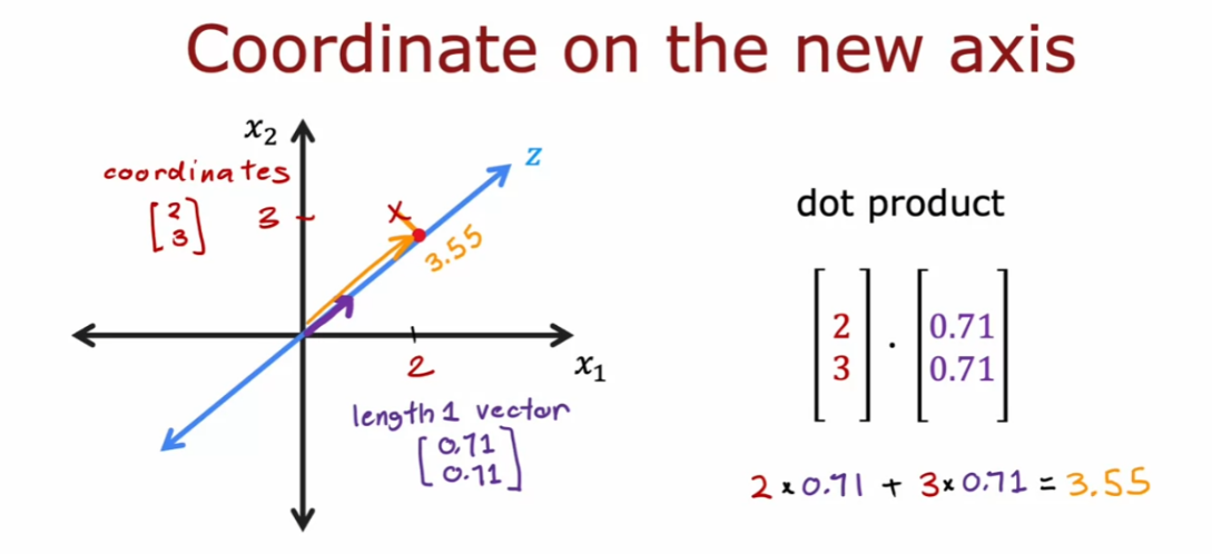
So far, we have talked about
how to use PCA to reduce data down to one dimension
or down to one number. We did so by finding the
principal component, also called sometimes the
first principal component. In this example, we had found
this as the first axis.

It turns out that if you
were to pick a second axis, the second axis
will always be at 90 degrees to the first axis. If you were to choose
even a third axis, then the third axis will be at 90 degrees to the first
and the second axis. By the way, in mathematics, 90 degrees is sometimes
called perpendicular.

The term perpendicular
just means at 90 degrees. Mathematicians will sometimes
say the second axis, z_2, is at 90 degrees or is
to the first axis, z_1. If you choose additional axes, they’re also at 90 degrees
or perpendicular to z_1 and z_2 and to any other
axes that PCA will choose.

If you had 50 features and wanted to find three
principal components, then if that’s the first axis, the second axis will be
at 90 degrees to it. Then the third axis will also be at 90 degrees to the first
and the second axis.

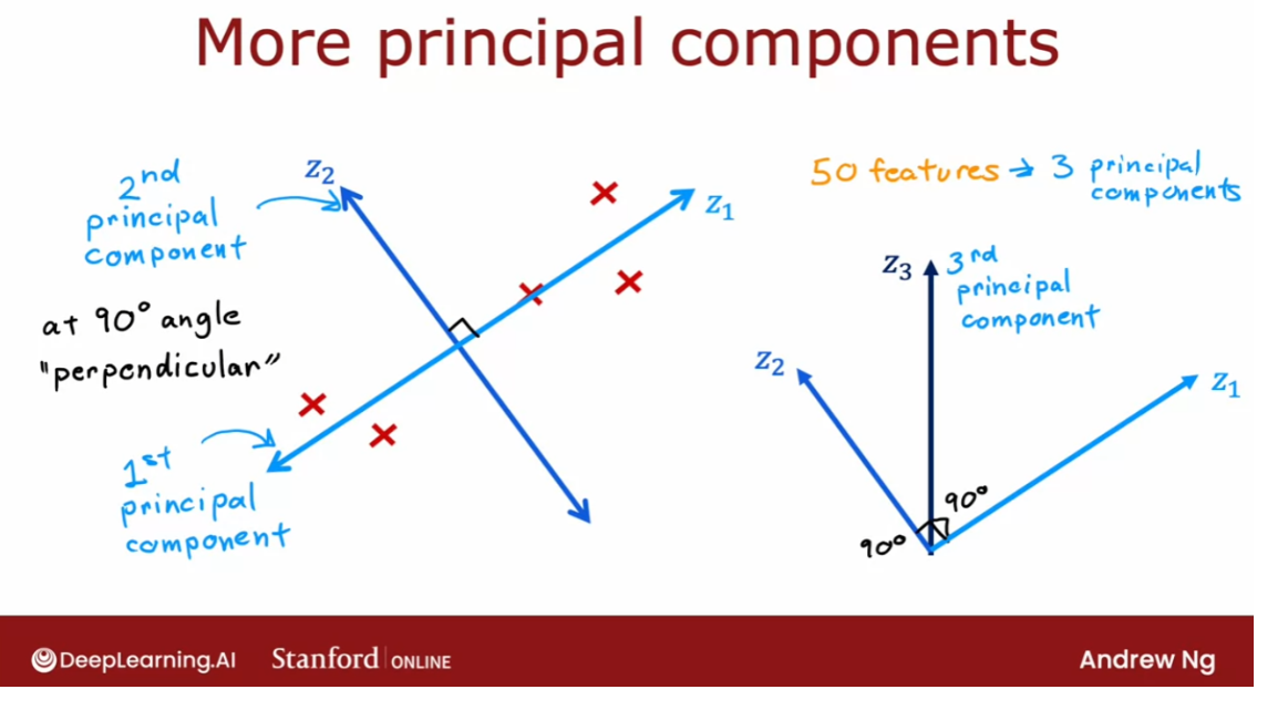
Now, one question
I’m often asked is, how is PCA different
from linear regression? It turns out PCA is
not linear regression, is a totally
different algorithm. Let me explain why.

With linear regression, which is a supervised
learning algorithm, you have data x and y. Here’s a data set where
the horizontal axis is the feature x and the vertical
axis here is the label y. With linear regression
you’re trying to fit a straight line so that the predicted value is as close as possible to the
ground truth label y. In other words, you’re trying
to minimize the length of these little line segments which are in the vertical direction. They just aligned
with the y axis.

In contrast, in PCA, there is no ground
truth label y. You just have unlabeled data, X1 and X2, and furthermore, you’re
not trying to fit a line to use X1 to predict X2. Instead, the average
treats X1 and X2 equally. We’re trying to
find this axis Z, that it turns out we end up making these little
line segments small when you project
the data onto Z.

In linear regression,
there is one number Y, which is given very
special treatment. We’re always trying
to measure distance between the fitted line and Y, which is why these distances are measured just in the
direction of the y-axis. Whereas in PCA, you can
have a lot of features, X1, X2, maybe all the way up to X50 if you
have 50 features. All 50 features are
treated equally. We’re just trying
to find an axis Z so that when the data is
projected onto the axis Z using these line
segments that you still retain as much of the variance of the original
data as possible.

I know that when I plot these
things in two-dimensions, we’ve just two
features, which is, I can draw on a flat
computer monitor. These arrows look like maybe they’re a
little bit similar. But when you have more
than two features, which is most of the case, the difference between
linear regression and PCA and what the algorithms
do is very large.

These algorithms are used for totally different purposes and give you very different answers. When linear regression
is used to predict a target output Y and
PCA is trying to take a lot of features and treat
them all equally and reduce the number of axis needed
to represent the data well. It turns out that maximizing the spread of these
projections will correspond to minimizing
the distances of these line segments, the distances to
the points have to move to be projected down to Z.

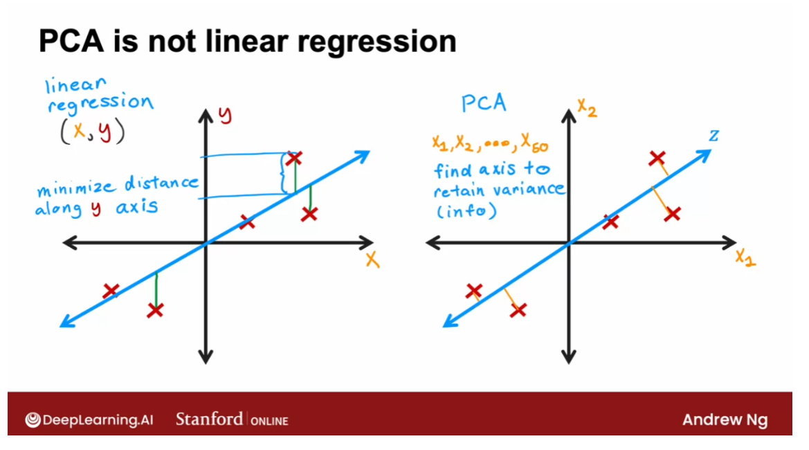
To illustrate the
difference between linear regression and
PCA in another way, if you have a data set
that looks like this, linear regression,
all it can do is fit a line that looks like that. Whereas if your data
set looks like this, PCA will choose this to be
the principal component. So you should use linear regression
if you’re trying to predict the value of y, and you should use PCA
if you’re trying to reduce the number of
features in your data set, say to visualize it.

Finally, before we
wrap up this video, there’s one more thing you
could do with PCA, which is, recall this example which
was at coordinates 2,3. We found that if you
projected to the z-axis, you end up with 3.55. One thing you could do is if you have an example
where Z equals 3.55, given just this one
number Z, 3.55, can we try to figure out what
was the original example?

It turns out that there’s a step in PCA called reconstruction, which is to try to go from
this one number Z equals 3.55 back to the original
two numbers, X1 and X2. It turns out you don’t
have enough information to get back X1 and X2 exactly, but you can try to
approximate it. In particular, the formula is, you would take this number 3.55, which is Z, and multiply it by the length one vector
that we had just now, which is 0.71, 0.71. This ends up to be 2.52, 2.52, which is this
point over here.

We can approximate the
original training example, which was a coordinates 2, 3 with this new point here, which is at 2.52, 2.52. The difference between
the original point and the projected point is this
little line segment here. In this case is not a
bad approximation 2.52, 2.52 is not that far from 2, 3. With just one number, we could get a reasonable
approximation to the coordinates of the
original training example. This is called the
reconstruction step of PCA.

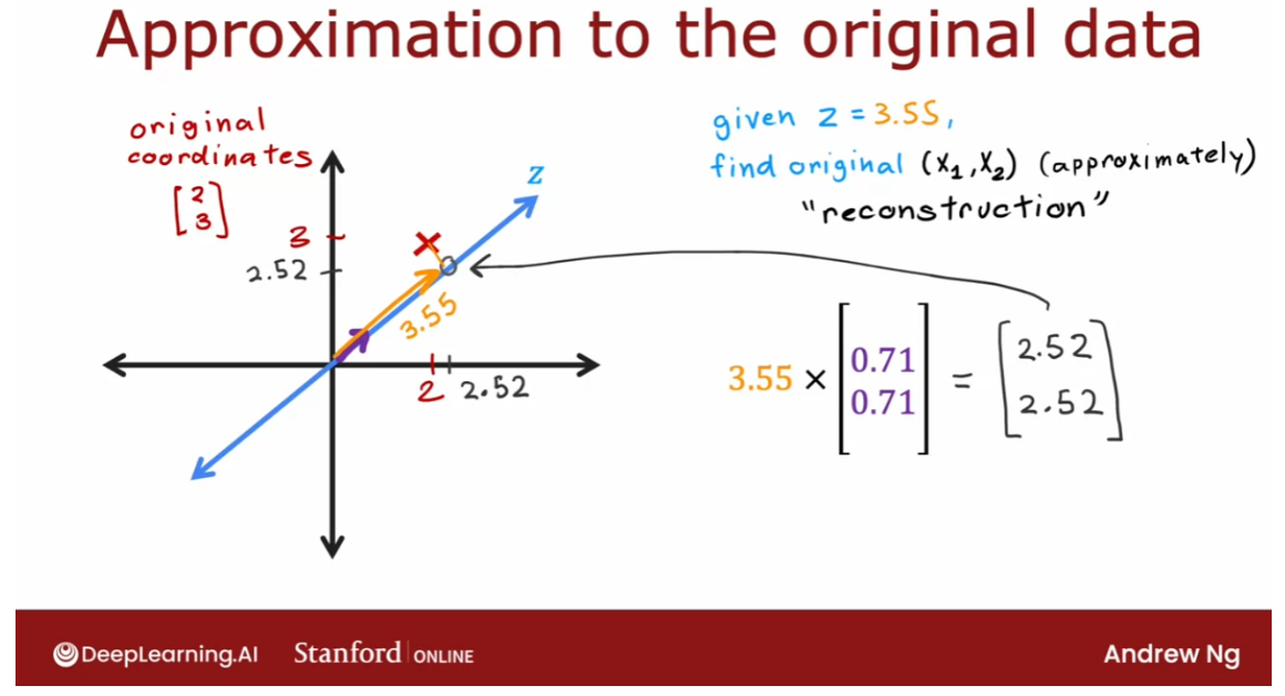
To summarize, the PCA
algorithm looks at your original data and
chooses one or more new axis, Z or maybe Z1 and Z2, to represent your
data and by taking your original data
set and projecting it onto your new axis or axis. This gives you a smaller
set of numbers so you can plot if wished to
visualize your data.

You’re seeing the math. Let’s now take a look at how you can implement this in code. In the next video, we’ll
look at how you can use PCA yourself using the
scikit-learn library. Let’s go on to the next video.

PCA in code (optional)

In this video, we’ll take a
look at how you can use the scikit-learn library
to implement PCA. These are the main steps. First, if your features take on very different
ranges of values, you can perform
pre-processing to scale the features to take on comparable ranges of values. If you were looking at the features of
different countries, those features take on very
different ranges of values. GDP could be in
trillions of dollars, whereas other features
are less than 100.

Feature scaling in applications
like that would be important to help PCA find a
good choice of axes for you. The next step then is to
run the PCA algorithm to “fit” the data to obtain
two or three new axes, Z_1, Z_2, and maybe Z_3. Here I’m assuming you want two or three axes if you want to visualize the
data in 2D or 3D. If you have an
application where you want more than two
or three axes, the PCA implementation can also give you more than
two or three axes, it’s just that it’d then
be harder to visualize. In scikit-learn, you will
use the fit function, or the fit method in
order to do this.

The fit function in PCA automatically carries
out mean normalization, it subtracts out the
mean of each feature. So you don’t need to separately perform
mean normalization. After running the fit function, you would get the new axes, Z_1, Z_2, maybe Z_3, and in PCA, we also call these the
principal components, where Z_1 is the first
principal component, Z_2 the second
principal component, and Z_3 the third
principal component.

After that, I would
recommend taking a look at how much each
of these new axes, or each of these new
principal components explains the variance
in your data. I’ll show a concrete example of what this means on
the next slide, but this lets you get a sense of whether
or not projecting the data onto these axes help you to retain most
of the variability, or most of the information
in the original dataset. This is done using the explained
variance ratio function.

Finally, you can transform, meaning just project the
data onto the new axes, onto the new
principal components, which you will do with
the transform method. Then for each training example, you would just have
two or three numbers, you can then plot those
two or three numbers to visualize your data.

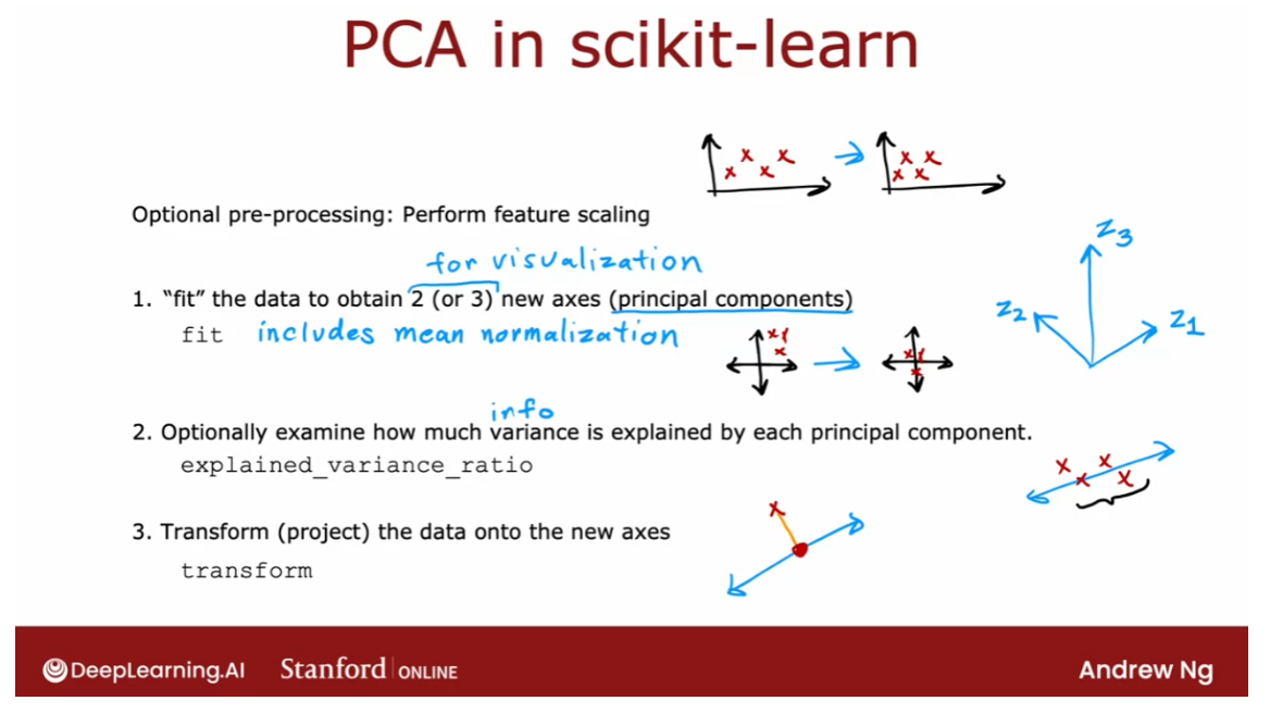
In detail, this is what
PCA in code looks like. Here’s the dataset X
with six examples. X equals NumPy array, the six examples over here. To run PCA to reduce this
data from two numbers, X_1, X_2 to just one number Z, you would run PCA and ask it to fit one principal component. N components here
is equal to one, and fit PCA to X. Pca_1 here is my notation for PCA with a single
principle component, with a single axis.

It turns out, if you
were to print out pca_1.explained_variance_ratio,
this is 0.992. This tells you that
in this example when you choose one axis, this captures 99.2 percent of the variability or of the information in
the original dataset.

Finally, if you want
to take each of these training samples and
project it to a single number, you would then call this, and this will output
this array with six numbers corresponding to
your six training examples. For example, the first
training example 1,1, projected to the
Z-axis gives you this number, 1.383, so on. So if you were to visualize this dataset using
just one dimension, this will be the number I use to represent
the first example.

The second example is projected to be this number and so on. I hope you take a
look at the optional lab where you see that these six examples
have been projected down onto this axis, onto this line which is now Y. All six examples now lie on this line that
looks like this. The first training example, which was 1,1, has been mapped to this example, which has a distance of
1.38 from the origin, so that’s why this is 1.38. Just one more quick example. This data is
two-dimensional data, and we reduced it
to one dimensions.

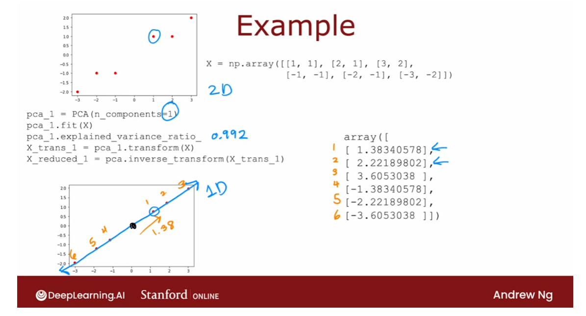
What if you were to compute
two principal components? Starts with two-dimensions, and then also end up
with two-dimensions. This isn’t that useful for visualization but it
might help us understand better how PCA and how
they code for PCA works. Here’s the same code
except that I’ve changed n components to two. I’m going to ask
the algorithm to find two principal components. If you do that the pca_2 explain ratio becomes 0.992, 0.008. What that means is that z_1, the first principle components, still continuous explain 99.2
percent of the variance, Z_2 the second
principle components, or the second axis, explains 0.8 percent
of the variance. These two numbers
together add up to one. Because while this data
is two-dimensional, so the two axes, Z_1 and Z_2, together they
explain 100 percent of the variance in the data.

If you were to
transform our project the data onto the
Z_1 and Z_2 axes, this is what you get, with now the first
training example is napped to these two numbers, corresponding to its
projection onto z_1, and z_2, and the second example, which is this projected
onto z_1 and z_2, becomes these two numbers. If you were to reconstruct the original data
roughly this is z_1, and this z_2, then the first training
example which was a [1, 1] has a distance of
1.38 on the z_1 axis, has this number and
the distance here of 0.29 hence this distance
on the z_2 axis, and the reconstruction
actually looks exactly the same as
the original data.

Because, if you
reduce or not really reduce two-dimensional data
to two-dimensional data, there is no approximation and you can get back to
your original dataset, with the projections
onto z_1 and z_2. This is what the code
to run PCA looks like. I hope you take a look at the optional lab where you can play with this more yourself. Also try varying the
parameters look at a specific example to deepen your intuition about
how PCA works.

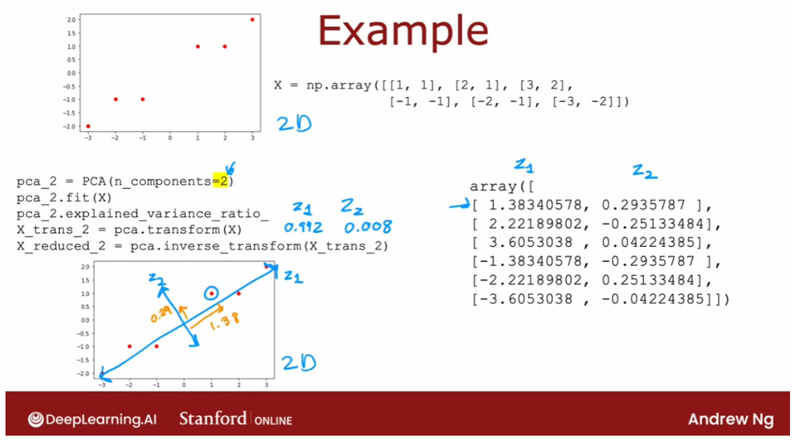
Before wrapping up,
I’d like to share a little bit of advice
for applying PCA. PCA is frequently used for
visualization where you reduce data to two or three
numbers so you can plot it. Like you saw in an earlier
video with the data on different countries so you can visualize
different countries. There are some other
applications of PCA that you may
occasionally hear about. That used to be more popular, maybe 10,15, 20 years ago
but much less so now.

Another possible use of
PCA is data compression. For example, if you have a database of lots
of different cars, and you have 50
features per car, but it’s just taking
up too much space on your database or maybe transmitting 50 numbers
over the Internet, just takes too long. Then one thing you
could do is reduce these 50 features to a
smaller number of features. It could be 10 features with 10 axes or 10
principal components. You can visualize 10-dimensional
data that easily, but this is 1/5 of
the storage space, or maybe 1/5 over the network
transmission costs needed. Many years ago I saw PCA use for this
application and more often, but today with modern storage being able to store
pretty large datasets and modern networking, able to transmit faster and
more data than ever before. I see this use much less often
as an application of PCA.

One of the applications
of PCA that again used to be more common
maybe 10 years ago, 20 years ago, but
much less so now is using it to speed up training of a supervised
learning model.

Where the idea is, if you had 1,000 features, and having a 1,000 features may the supervised learning
algorithm runs too slowly. Maybe you can reduce it
to 100 features using PCA and then your dataset is
basically smaller and your supervised learning
algorithm may run faster. This used to make a difference
in the running time of some of the older generations
of learning algorithms, such as if you have had a
support vector machines. This will speed up a
support vector machine.

But it turns out with modern
machine learning algorithms, algorithms like deep learning, this doesn’t actually
help that much, and is much more common to just take the
high-dimensional dataset, and feed it into say
your neural network. Rather than run PCA because PCA has some computational
cost as well. You may hear about this in some of the older research papers, but I don’t really see
this done much anymore. But the most common
thing that I use PCA for today is
visualization and then I find it very useful to reduce the dimensional data
to visualize it.

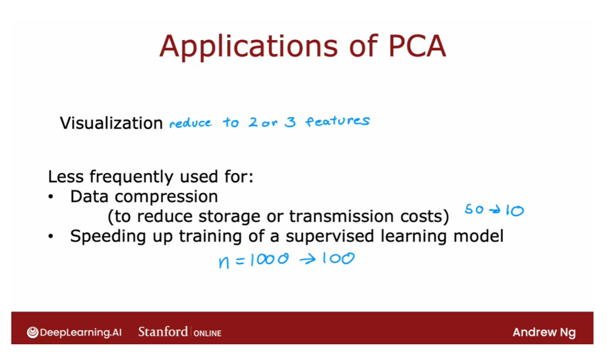
Thanks for sticking
with me through the end of the optional
videos for this week, I hope you enjoy learning about PCA and that you
find a useful when you get a new
dataset for reducing the dimension of the dataset
to two or three dimensions so you can visualize
it and hopefully gain new insights
into your data sets. There’s helped me many times understand my own datasets and I hope that you find it
equally useful as well. Thanks for watching
these videos and I look forward to
seeing you next week.

Lab: PCA and data visualization (optional)

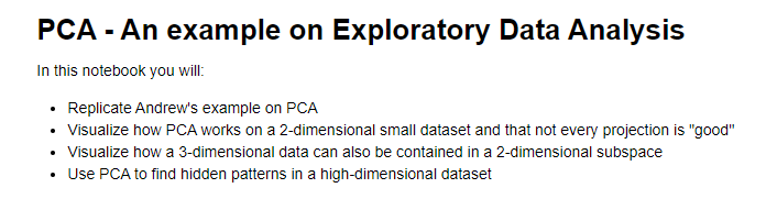
这是一个可选的lab，没有要写的代码，所以这里就不放出来了。

其他

提交到github仓库的一些模板

git commit -m "Finish optional PCA notes of week 02 of Unsupervised Learning, Recommenders, Reinforcement Learning. Notes of week 02 done!"

How do you do this efficiently computationally 两个副词

perpendicular to 垂直于

后记

花费两天时间完成week2的学习与记录。

这篇关于机器学习专项课程03：Unsupervised Learning, Recommenders, Reinforcement Learning笔记 Week02的文章就介绍到这儿，希望我们推荐的文章对编程师们有所帮助！

---