CS231n-2017 Assignment3 RNN、LSTM、风格迁移

本文主要是介绍CS231n-2017 Assignment3 RNN、LSTM、风格迁移，希望对大家解决编程问题提供一定的参考价值，需要的开发者们随着小编来一起学习吧！

一、RNN

所需完成的步骤记录在RNN_Captioning.ipynb文件中。

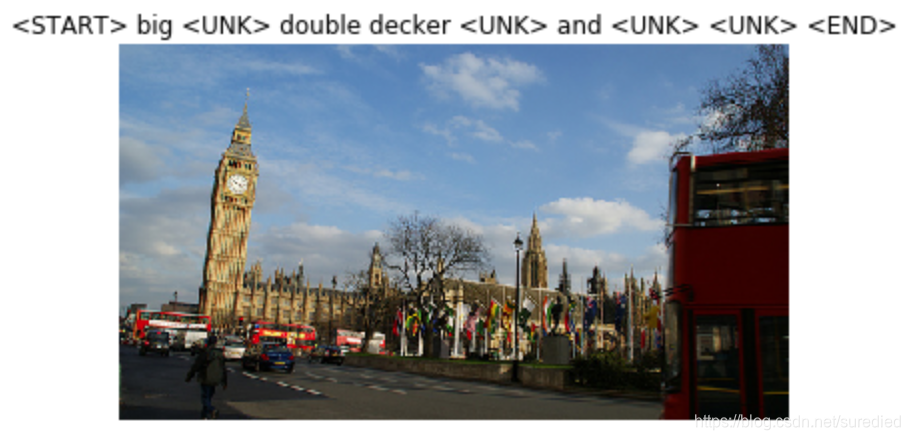
本例中所用的数据为Microsoft于2014年发布的COCO数据集。该数据集中和图像标注想拐的图片包含80000张训练图片和40000张验证图片。而这些图片的特征已通过VGG-16网络获得，存储在train2014_vgg16_fc7.h5和val2014_vgg16_fc7.h5文件中，每张图片由一个4096维的向量表征。为减少问题复杂度，本例还提供了经过PCA处理之后的特征，存储在train2014_vgg16_fc7_pca.h5和val2014_vgg16_fc7_pca.h5文件中，特征维度由4096维降低为512维。

图片和其标注示例如下，其中<START>和<END>为标注的起始和结束字符，<UNK>为词表中未出现的罕见词，另外为保证标注的长度一致，会在较短的标注后填充<NULL>特殊字符。

1. RNN的单步前向传播

前向传播的实现的方式，与上次作业大同小异，只不过这里将会实现循环网络层的逻辑。
考虑每次网络读入一个标注词时，将根据此次输入和此时的网络隐藏状态，计算新的网络隐藏状态。

rnn_layers.py文件中的rnn_step_forward()函数：

def rnn_step_forward(x, prev_h, Wx, Wh, b):next_h, cache = None, None# TODO: Implement a single forward step for the vanilla RNN. next_h = tanh(np.dot(x, Wx) + np.dot(prev_h, Wh) + b)cache = (next_h, Wx, Wh, x, prev_h)return next_h, cache

其中tanh()为求取超正切值的辅助函数，一个考虑计算溢出异常的稳定版本如下：

def tanh(x):tmp = x.copy()tmp[tmp > 10] = 10tmp = np.exp(tmp*2)return (tmp - 1)/(tmp + 1)

2. RNN的单步反向传播

关于超正切函数的求导：

$$\tanh x=\frac{e^x-e^{-x}}{e^x+e^{-x}}\Rightarrow {\tanh }^{\prime }x=1-{\tanh }^{2}x$$
故在rnn_layers.py文件中实现rnn_step_backward()函数如下：

def rnn_step_backward(dnext_h, cache):dx, dprev_h, dWx, dWh, db = None, None, None, None, None# TODO: Implement the backward pass for a single step of a vanilla RNN. next_h, Wx, Wh, x, prev_h = cachedtanh_h = dnext_h * (1 - next_h**2)dx = dtanh_h.dot(Wx.T)dprev_h = dtanh_h.dot(Wh.T)dWx = x.T.dot(dtanh_h)dWh = prev_h.T.dot(dtanh_h)db = np.sum(dtanh_h, axis=0)return dx, dprev_h, dWx, dWh, db

3. RNN的前向传播

网络读取一小批的标注数据x，(样本数为N，每条标注的长度为T)，并使用这批标注所对应图片的特征作为网络的初始隐藏状态h0，通过前向传播过程，获得各个样本在每一步推进中产生的隐藏状态h，并存储反向传播所需变量。
rnn_layers.py文件中的rnn_forward()函数：

def rnn_forward(x, h0, Wx, Wh, b):h, cache = None, None# TODO: Implement forward pass for a vanilla RNN running on a sequence of input data.N, T, D = x.shape_, H = h0.shapeh = np.zeros((N, T, H))prev_h = h0for iter_time in range(T):h[:, iter_time, :],_ = rnn_step_forward(x[:, iter_time, :], prev_h, Wx, Wh, b)prev_h = h[:, iter_time, :]cache = (h0, h, Wx, Wh, x)return h, cache

4. RNN的反向传播

利用存储的变量实现反向传播过程。rnn_layers.py文件中的rnn_backward()函数：

def rnn_backward(dh, cache):dx, dh0, dWx, dWh, db = None, None, None, None, None# TODO: Implement the backward pass for a vanilla RNN running an entire sequence of data.N, T, H = dh.shapeh0, h, Wx, Wh, x = cachedh0 = np.zeros_like(h0)dx = np.zeros_like(x)dWx = np.zeros_like(Wx)dWh = np.zeros_like(Wh)db = np.zeros(H)h = np.concatenate((h0[:, np.newaxis, :], h), axis=1)for iter_time in range(T):dnext_h = dh[:, -(iter_time+1), :] + dh0cache = (h[:, -(iter_time+1), :], Wx, Wh, x[:, -(iter_time+1), :], h[:, -(iter_time+2), :])dx_step, dh0, dWx_step, dWh_step, db_step = rnn_step_backward(dnext_h, cache)dx[:, -(iter_time+1), :] = dx_stepdWx += dWx_stepdWh += dWh_stepdb  += db_stepreturn dx, dh0, dWx, dWh, db

注意其中梯度值的累积，这其实就是RNN共享参数的一种体现。

5. 字词的向量化表达

将图像标注中的词索引x转化为向量表达，并在后向传播时更新字词所对应的向量。
rnn_layers.py文件中的word_embedding_forward()函数：

def word_embedding_forward(x, W):out, cache = None, None# TODO: Implement the forward pass for word embeddings.out = W[x, :]cache = (x, W.shape)return out, cache

rnn_layers.py文件中的word_embedding_backward()函数：

def word_embedding_backward(dout, cache):dW = None# TODO: Implement the backward pass for word embeddings.x, shp = cachedW = np.zeros(shp)np.add.at(dW, x, dout)return dW

6. 考虑损失函数

rnn.py文件中的loss()函数：

def loss(self, features, captions):captions_in = captions[:, :-1]captions_out = captions[:, 1:]# You'll need thismask = (captions_out != self._null)# Weight and bias for the affine transform from image features to initial# hidden stateW_proj, b_proj = self.params['W_proj'], self.params['b_proj']# Word embedding matrixW_embed = self.params['W_embed']# Input-to-hidden, hidden-to-hidden, and biases for the RNNWx, Wh, b = self.params['Wx'], self.params['Wh'], self.params['b']# Weight and bias for the hidden-to-vocab transformation.W_vocab, b_vocab = self.params['W_vocab'], self.params['b_vocab']loss, grads = 0.0, {}############################################################################# TODO: Implement the forward and backward passes for the CaptioningRNN.h0, cache_affine = affine_forward(features, W_proj, b_proj)  # (1)captions_in_vec, cache_embed = word_embedding_forward(captions_in, W_embed)  #(2)if self.cell_type == "rnn":h, cache_rnn = rnn_forward(captions_in_vec, h0, Wx, Wh, b)  # (3)elif self.cell_type == "lstm":h, cache_lstm = lstm_forward(captions_in_vec, h0, Wx, Wh, b)scores, cache_score = temporal_affine_forward(h, W_vocab, b_vocab)  # (4)loss, dscores = temporal_softmax_loss(scores, captions_out, mask)  # (5)dh, dW_vocab, db_vocab = temporal_affine_backward(dscores, cache_score) # (4)if self.cell_type == "rnn":dcaptions_in_vec, dh0, dWx, dWh, db = rnn_backward(dh, cache_rnn)  # (3)elif self.cell_type == "lstm":dcaptions_in_vec, dh0, dWx, dWh, db = lstm_backward(dh, cache_lstm)  # (3)dW_embed = word_embedding_backward(dcaptions_in_vec, cache_embed)  # (2)_, dW_proj, db_proj = affine_backward(dh0, cache_affine)  # (1)grads = {"W_vocab": dW_vocab, "b_vocab": db_vocab, "Wx": dWx, "Wh": dWh, "b": db,"W_embed": dW_embed, "W_proj": dW_proj, "b_proj": db_proj}return loss, grads

7. 测试过程

rnn.py文件中的sample()函数：

def sample(self, features, max_length=30):N = features.shape[0]captions = self._null * np.ones((N, max_length), dtype=np.int32)# Unpack parametersW_proj, b_proj = self.params['W_proj'], self.params['b_proj']W_embed = self.params['W_embed']Wx, Wh, b = self.params['Wx'], self.params['Wh'], self.params['b']W_vocab, b_vocab = self.params['W_vocab'], self.params['b_vocab']# TODO: Implement test-time sampling for the model.c = np.zeros(b.shape[0]//4)h = features.dot(W_proj) + b_proj  # (1)captions[:, 0] = self._startfor iter_time in range(1, max_length):prev_word = captions[:, iter_time-1]captions_in_vec, _ = word_embedding_forward(prev_word, W_embed)  #(2)if self.cell_type == "rnn":h, _ = rnn_step_forward(captions_in_vec, h, Wx, Wh, b)  # (3)else:h, c, _ = lstm_step_forward(captions_in_vec, h, c, Wx, Wh, b)  # (3)scores =  np.dot(h, W_vocab) + b_vocab  # (4)captions[:, iter_time] = np.argmax(scores, axis=1)passreturn captions

二、LSTM

所需完成的步骤记录在LSTM_Captioning.ipynb文件中。

1. LSTM的单步前向传播

rnn_layers.py文件中的lstm_step_forward()函数：

def lstm_step_forward(x, prev_h, prev_c, Wx, Wh, b):next_h, next_c, cache = None, None, None# TODO: Implement the forward pass for a single timestep of an LSTM.H = b.shape[0]ifog = x.dot(Wx) + prev_h.dot(Wh) + bifog = getIFOG(ifog, "T")next_c = getIFOG(ifog, 'f')*prev_c + getIFOG(ifog,'i')*getIFOG(ifog,"g")next_h = getIFOG(ifog, 'o')*tanh(next_c)cache = (x, prev_h, prev_c, Wx, Wh, next_c, ifog)return next_h, next_c, cache

其中getIFOG()函数为变换并拆分四门输出的辅助函数：

def getIFOG(ifog, which):H = ifog.shape[1]//4indx = {char:i*H for i, char in enumerate("ifog")}if which == "t" or which == "T":for char in indx:if char == "g":ifog[:, indx[char]:indx[char]+H] = tanh(ifog[:, indx[char]:indx[char]+H])else:ifog[:, indx[char]:indx[char]+H] = sigmoid(ifog[:, indx[char]:indx[char]+H])return ifogelse:if which == "g":return ifog[:, indx[which]:indx[which]+H]else:return ifog[:, indx[which]:indx[which]+H]

2. LSTM的单步后向传播

rnn_layers.py文件中实现lstm_step_backward()函数：

def lstm_step_backward(dnext_h, dnext_c, cache):dx, dh, dc, dWx, dWh, db = None, None, None, None, None, None# TODO: Implement the backward pass for a single timestep of an LSTM.N, H = dnext_c.shapeda = np.zeros((N, 4*H))x, prev_h, prev_c, Wx, Wh, next_c, ifog = cachetanhc_t = tanh(next_c)i = getIFOG(ifog, "i")f = getIFOG(ifog, "f")o = getIFOG(ifog, "o")g = getIFOG(ifog, "g")dh_c = dnext_h*o*(1-tanhc_t**2)setIFOG(da, "i", (dnext_c + dh_c)*g*(1-i)*i)setIFOG(da, "f", (dnext_c + dh_c)*prev_c*(1-f)*f)setIFOG(da, "o", dnext_h*tanhc_t*(1-o)*o)setIFOG(da, "g", (dnext_c + dh_c)*i*(1-g**2))dx = da.dot(Wx.T)dprev_h = da.dot(Wh.T)dprev_c = (dnext_c + dh_c) * fdWx = x.T.dot(da)dWh = prev_h.T.dot(da)db = np.sum(da, axis=0)return dx, dprev_h, dprev_c, dWx, dWh, db

由实现过程可见：LSTM中反馈到前一层的梯度除了dprev_h外，还包含dprev_c。其中dprev_h涉及与系数矩阵W的相乘，因此这一项在经历多步操作时，极易出现梯度爆炸或消失。而dprev_c这一项，只涉及元素相乘，因此，缓解了上述问题。

3. LSTM的前向传播

rnn_layers.py文件中的lstm_forward()函数：

def lstm_forward(x, h0, Wx, Wh, b):h, cache = None, None# TODO: Implement the forward pass for an LSTM over an entire timeseries.N, T, D = x.shape_, H = h0.shapeh = np.zeros((N, T, H))c = np.zeros_like(h)prev_h = h0prev_c = np.zeros_like(prev_h)for iter_time in range(T):h[:, iter_time, :], c[:, iter_time, :], _ = lstm_step_forward(x[:, iter_time, :], prev_h, prev_c, Wx, Wh, b)prev_h = h[:, iter_time, :]prev_c = c[:, iter_time, :]cache = (h0, h, c, Wx, Wh, x, b)return h, cache

4. LSTM的反向传播

rnn_layers.py文件中的lstm_backward()函数：

def lstm_backward(dh, cache):dx, dh0, dWx, dWh, db = None, None, None, None, None# TODO: Implement the backward pass for an LSTM over an entire timeseries.h0, h, c, Wx, Wh, x, b = cacheN, T, H = dh.shapedh0 = np.zeros_like(h0)dx = np.zeros_like(x)dWx = np.zeros_like(Wx)dWh = np.zeros_like(Wh)db = np.zeros(4*H)h = np.concatenate((h0[:, np.newaxis, :], h), axis=1)dnext_c = np.zeros_like(h0)c = np.concatenate((dnext_c[:, np.newaxis, :], c), axis=1)for iter_time in range(T):dnext_h = dh[:, -(iter_time+1), :] + dh0prev_h = h[:, -(iter_time+2), :]next_x = x[:, -(iter_time+1), :]ifog = next_x.dot(Wx) + prev_h.dot(Wh) + bifog = getIFOG(ifog, "T")cache = (next_x, prev_h, c[:, -(iter_time+2), :], Wx, Wh, c[:, -(iter_time+1), :], ifog)dx_step, dh0, dnext_c, dWx_step, dWh_step, db_step = lstm_step_backward(dnext_h, dnext_c, cache)dx[:, -(iter_time+1), :] = dx_stepdWx += dWx_stepdWh += dWh_stepdb  += db_stepreturn dx, dh0, dWx, dWh, db

三、网络的可视化

所需完成的步骤记录在NetworkVisualization-PyTorch.ipynb文件中(作业代码包里还提供了一个TensorFlow版本)。

在本部分中，将使用一个预训练的分类网络，来完成显著图显示、生成某类别的图像等任务。该预训练的网络是在ImageNet数据集上得到的SqueezeNet，其可得到与AlexNet相当的精度，但参数规模小到足以在CPU机器上完成本部分的工作。

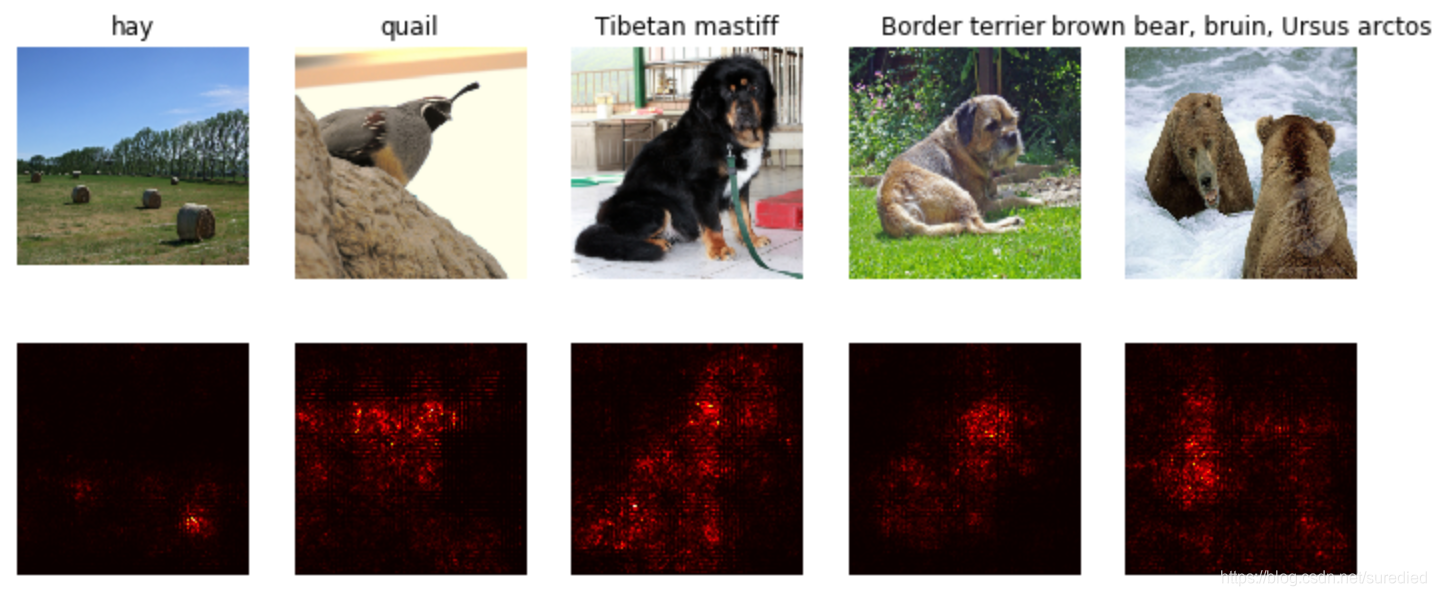
1. 显著图

显著图(Saliency Map)展示了图像各部分对最终分类结果的影响程度。其计算方式是：网络终端的该图像的正确类别的得分对于图像像素的梯度。

NetworkVisualization-PyTorch.ipynb中的compute_saliency_maps函数：

def compute_saliency_maps(X, y, model):# Make sure the model is in "test" modemodel.eval()# Wrap the input tensors in VariablesX_var = Variable(X, requires_grad=True)y_var = Variable(y)saliency = None# TODO: Implement this function.y_pred = model(X_var)scores = y_pred.gather(1, y_var.view(-1, 1)).squeeze()loss = scores.sum()loss.backward()saliency = torch.max(torch.abs(X_var.grad), 1)[0]passreturn saliency

在若干图片上的计算结果：

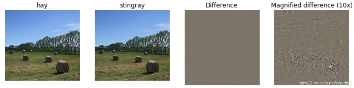
2. 愚弄分类器

计算某图片在一个错误分类上的得分关于图片各像素的梯度，然后使用梯度上升法，修改图片，使得网络发生误判。
NetworkVisualization-PyTorch.ipynb中的make_fooling_image函数：

def make_fooling_image(X, target_y, model):# Initialize our fooling image to the input image, and wrap it in a Variable.X_fooling = X.clone()X_fooling_var = Variable(X_fooling, requires_grad=True)learning_rate = 1# TODO: Generate a fooling image X_fooling that the model will classify as the class target_y. score = model(X_fooling_var)_, y_pred = torch.max(score,1)iter_count = 0while(y_pred.item() != target_y):iter_count += 1if iter_count%10 == 0:print(iter_count)loss = score[0, target_y]loss.backward()g = X_fooling_var.grad/X_fooling_var.grad.norm()X_fooling += learning_rate * gX_fooling_var.grad.zero_()model.zero_grad()score = model(X_fooling_var)_, y_pred = torch.max(score,1)print(iter_count)return X_fooling

最终生成的使网络误判的图片与原图的差异示例如下：

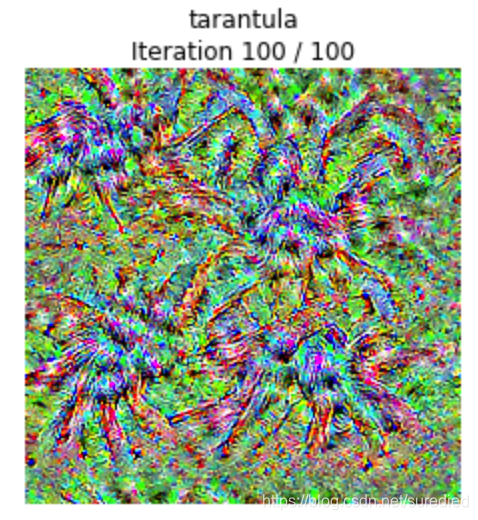
3. 生成最符合某类别的图片

优化目标函数定为某分类的得分再加上正则项；将图片初始为随机噪声，使用梯度上升法，生成最符合该类别的图片。

NetworkVisualization-PyTorch.ipynb中的create_class_visualization函数：

def create_class_visualization(target_y, model, dtype, **kwargs):model.type(dtype)l2_reg = kwargs.pop('l2_reg', 1e-3)learning_rate = kwargs.pop('learning_rate', 25)num_iterations = kwargs.pop('num_iterations', 100)blur_every = kwargs.pop('blur_every', 10)max_jitter = kwargs.pop('max_jitter', 16)show_every = kwargs.pop('show_every', 25)# Randomly initialize the image as a PyTorch Tensor, and also wrap it in# a PyTorch Variable.img = torch.randn(1, 3, 224, 224).mul_(1.0).type(dtype)img_var = Variable(img, requires_grad=True)for t in range(num_iterations):# Randomly jitter the image a bit; this gives slightly nicer resultsox, oy = random.randint(0, max_jitter), random.randint(0, max_jitter)img.copy_(jitter(img, ox, oy))# TODO: Use the model to compute the gradient of the score for the     ## class target_y with respect to the pixels of the image, and make a   ## gradient step on the image using the learning rate.score = model(img_var)loss = score[0, target_y] - l2_reg * img.norm()**2loss.backward()img += learning_rate*img_var.gradimg_var.grad.zero_()model.zero_grad()# Undo the random jitterimg.copy_(jitter(img, -ox, -oy))# As regularizer, clamp and periodically blur the imagefor c in range(3):lo = float(-SQUEEZENET_MEAN[c] / SQUEEZENET_STD[c])hi = float((1.0 - SQUEEZENET_MEAN[c]) / SQUEEZENET_STD[c])img[:, c].clamp_(min=lo, max=hi)if t % blur_every == 0:blur_image(img, sigma=0.5)# Periodically show the imageif t == 0 or (t + 1) % show_every == 0 or t == num_iterations - 1:plt.imshow(deprocess(img.clone().cpu()))class_name = class_names[target_y]plt.title('%s\nIteration %d / %d' % (class_name, t + 1, num_iterations))plt.gcf().set_size_inches(4, 4)plt.axis('off')plt.show()return deprocess(img.cpu())

对狼蛛类别的一个反演结果如下所示：

四、风格迁移

风格迁移问题的损失函数由三部分构成：

• 内容偏差：该部分由生成图片和源内容图片，在特征空间中的差异描述。

  StyleTransfer-PyTorch.ipynb中的content_loss()函数：

  def content_loss(content_weight, content_current, content_original):lc = content_weight * (content_current - content_original).norm()**2return lc
  

• 风格偏差：该部分由生成图片和源风格图片的Gram矩阵之间的差异描述。

  StyleTransfer-PyTorch.ipynb中的gram_matrix()函数：

  def gram_matrix(features, normalize=True):N, C, H, W = features.shapegram = Variable(torch.zeros(N, C, C))x = features.view(N, C, -1)for i in range(N):gram[i] = torch.mm(x[i], x[i].t())if normalize:gram = gram/H/W/Creturn gram
  

  StyleTransfer-PyTorch.ipynb中的style_loss()函数：

  def style_loss(feats, style_layers, style_targets, style_weights):style_loss = Variable(torch.FloatTensor([0]))for i, indx in enumerate(style_layers):gram = gram_matrix(feats[indx])style_loss += style_weights[i] * torch.sum((gram - style_targets[i]).norm()**2)return style_loss
  

注意其中style_loss应初始化为torch.Variable，以记录与其相关的运算，用于反向传播时梯度的累积。

• 图像变分惩罚项：该部分描述了图像的平滑度。

  StyleTransfer-PyTorch.ipynb中的tv_loss()函数：

  def tv_loss(img, tv_weight):x = torch.sum((img[:, :, 1:, :] - img[:, :, 0:-1, :]).norm()**2) + torch.sum((img[:, :, :, 1:] - img[:, :, :, 0:-1]).norm()**2)return tv_weight * xs
  

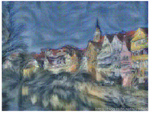
一个以梵高的星空为风格的迁移示例如下：

这篇关于CS231n-2017 Assignment3 RNN、LSTM、风格迁移的文章就介绍到这儿，希望我们推荐的文章对编程师们有所帮助！

---