本文主要是介绍Basic classification: Classify images of clothing,希望对大家解决编程问题提供一定的参考价值,需要的开发者们随着小编来一起学习吧!
tf_classification
1.数据读取,然后对数据进行预处理,把 x 转化成 float-point,y 还是保留 label 形式
2.搭建模型,要指定输入的 input_shape
3.compile 里面要指定 optimizer,loss_function,metric
4.对模型进行评估,预测的输出要经过 softmax 得到 probability 形式的表示
唯一有特点的地方是对预测的输出做了可视化处理
原始数据的像素值取值 [0, 255],需要转化成 [0, 1]
数据集是衣服,也就是说我们要对衣服进行分类
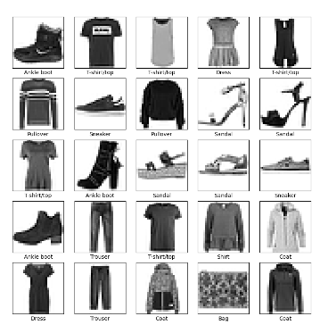
This guide uses the Fashion MNIST dataset which contains 70,000 grayscale images in 10 categories. The images show individual articles of clothing at low resolution (28 by 28 pixels), as seen here:
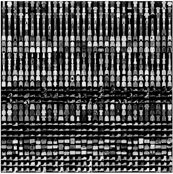
Fashion MNIST is intended as a drop-in replacement for the classic MNIST dataset
The images are 28x28 NumPy arrays, with pixel values ranging from 0 to 255. The labels are an array of integers, ranging from 0 to 9. These correspond to the class of clothing the image represents:
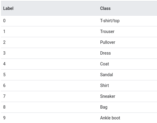
Each image is mapped to a single label. Since the class names are not included with the dataset, store them here to use later when plotting the images:
class_names = ['T-shirt/top', 'Trouser', 'Pullover', 'Dress', 'Coat','Sandal', 'Shirt', 'Sneaker', 'Bag', 'Ankle boot']
这里的 train label 是 0-9,class index 也是 0-9,然后 class index 和 class name 也能对应的上
# TensorFlow and tf.keras
import tensorflow as tf# Helper libraries
import numpy as np
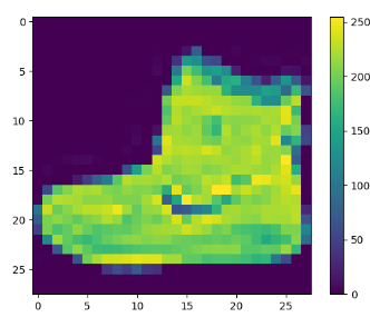
import matplotlib.pyplot as pltprint(tf.__version__)fashion_mnist = tf.keras.datasets.fashion_mnist(train_images, train_labels), (test_images, test_labels) = fashion_mnist.load_data()class_names = ['T-shirt/top', 'Trouser', 'Pullover', 'Dress', 'Coat','Sandal', 'Shirt', 'Sneaker', 'Bag', 'Ankle boot']# The data must be preprocessed before training the network. If you inspect the first image in the training set, you will see that the pixel values fall in the range of 0 to 255:
plt.figure()
plt.imshow(train_images[0])
plt.colorbar()
plt.grid(False)
plt.show()# Scale these values to a range of 0 to 1 before feeding them to the neural network model. To do so, divide the values by 255. It's important that the training set and the testing set be preprocessed in the same way:
train_images = train_images / 255.0test_images = test_images / 255.0plt.figure(figsize=(10, 10))
for i in range(25):plt.subplot(5, 5, i + 1)plt.xticks([])plt.yticks([])plt.grid(False)plt.imshow(train_images[i], cmap=plt.cm.binary)plt.xlabel(class_names[train_labels[i]])
plt.show()
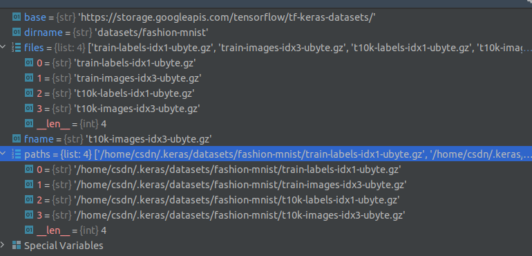
查了下 load_data() 的源码:

把 paths 展示了下
Building the neural network requires configuring the layers of the model, then compiling the model.
The basic building block of a neural network is the layer. Layers extract representations from the data fed into them. Hopefully, these representations are meaningful for the problem at hand.
Most of deep learning consists of chaining together simple layers. Most layers, such as tf.keras.layers.Dense, have parameters that are learned during training.
model = tf.keras.Sequential([tf.keras.layers.Flatten(input_shape=(28, 28)),tf.keras.layers.Dense(128, activation='relu'),tf.keras.layers.Dense(10)
])
The first layer in this network, tf.keras.layers.Flatten, transforms the format of the images from a two-dimensional array (of 28 by 28 pixels) to a one-dimensional array (of 28 * 28 = 784 pixels). Think of this layer as unstacking rows of pixels in the image and lining them up. This layer has no parameters to learn; it only reformats the data.
After the pixels are flattened, the network consists of a sequence of two tf.keras.layers.Dense layers. These are densely connected, or fully connected, neural layers. The first Dense layer has 128 nodes (or neurons). The second (and last) layer returns a logits array with length of 10. Each node contains a score that indicates the current image belongs to one of the 10 classes.
Before the model is ready for training, it needs a few more settings. These are added during the model’s compile step:
- Loss function —This measures how accurate the model is during training. You want to minimize this function to “steer” the model in the right direction.
- Optimizer —This is how the model is updated based on the data it sees and its loss function.
- Metrics —Used to monitor the training and testing steps. The following example uses accuracy, the fraction of the images that are correctly classified.
model.compile(optimizer='adam',loss=tf.keras.losses.SparseCategoricalCrossentropy(from_logits=True),metrics=['accuracy'])
Training the neural network model requires the following steps:
- Feed the training data to the model. In this example, the training data is in the train_images and train_labels arrays.
- The model learns to associate images and labels.
- You ask the model to make predictions about a test set—in this example, the test_images array.
- Verify that the predictions match the labels from the test_labels array.
test_loss, test_acc = model.evaluate(test_images, test_labels, verbose=2)print('\nTest accuracy:', test_acc)
It turns out that the accuracy on the test dataset is a little less than the accuracy on the training dataset. This gap between training accuracy and test accuracy represents overfitting. Overfitting happens when a machine learning model performs worse on new, previously unseen inputs than it does on the training data. An overfitted model “memorizes” the noise and details in the training dataset to a point where it negatively impacts the performance of the model on the new data. For more information, see the following:
-
Demonstrate overfitting
-
Strategies to prevent overfitting
With the model trained, you can use it to make predictions about some images. The model’s linear outputs, logits. Attach a softmax layer to convert the logits to probabilities, which are easier to interpret.
probability_model = tf.keras.Sequential([model,tf.keras.layers.Softmax()])predictions = probability_model.predict(test_images)
A prediction is an array of 10 numbers. They represent the model’s “confidence” that the image corresponds to each of the 10 different articles of clothing. You can see which label has the highest confidence value:
np.argmax(predictions[0])
Note that the model can be wrong even when very confident.
tf.keras models are optimized to make predictions on a batch, or collection, of examples at once. Accordingly, even though you’re using a single image, you need to add it to a list:
# Grab an image from the test dataset.
img = test_images[1]print(img.shape)# Add the image to a batch where it's the only member.
img = (np.expand_dims(img,0))print(img.shape)
最后把完整的代码片段放上来
# TensorFlow and tf.keras
import tensorflow as tf# Helper libraries
import numpy as np
import matplotlib.pyplot as pltprint(tf.__version__)fashion_mnist = tf.keras.datasets.fashion_mnist(train_images, train_labels), (test_images, test_labels) = fashion_mnist.load_data()class_names = ['T-shirt/top', 'Trouser', 'Pullover', 'Dress', 'Coat','Sandal', 'Shirt', 'Sneaker', 'Bag', 'Ankle boot']plt.figure()
plt.imshow(train_images[0])
plt.colorbar()
plt.grid(False)
plt.show()train_images = train_images / 255.0test_images = test_images / 255.0plt.figure(figsize=(10, 10))
for i in range(25):plt.subplot(5, 5, i + 1)plt.xticks([])plt.yticks([])plt.grid(False)plt.imshow(train_images[i], cmap=plt.cm.binary)plt.xlabel(class_names[train_labels[i]])
plt.show()model = tf.keras.Sequential([tf.keras.layers.Flatten(input_shape=(28, 28)),tf.keras.layers.Dense(128, activation='relu'),tf.keras.layers.Dense(10)
])model.compile(optimizer='adam',loss=tf.keras.losses.SparseCategoricalCrossentropy(from_logits=True),metrics=['accuracy'])model.fit(train_images, train_labels, epochs=10)test_loss, test_acc = model.evaluate(test_images, test_labels, verbose=2)print('\nTest accuracy:', test_acc)probability_model = tf.keras.Sequential([model,tf.keras.layers.Softmax()])predictions = probability_model.predict(test_images)print(np.argmax(predictions[0]))
print(test_labels[0])def plot_image(i, predictions_array, true_label, img):true_label, img = true_label[i], img[i]plt.grid(False)plt.xticks([])plt.yticks([])plt.imshow(img, cmap=plt.cm.binary)predicted_label = np.argmax(predictions_array)if predicted_label == true_label:color = 'blue'else:color = 'red'plt.xlabel("{} {:2.0f}% ({})".format(class_names[predicted_label],100 * np.max(predictions_array),class_names[true_label]),color=color)def plot_value_array(i, predictions_array, true_label):true_label = true_label[i]plt.grid(False)plt.xticks(range(10))plt.yticks([])thisplot = plt.bar(range(10), predictions_array, color="#777777")plt.ylim([0, 1])predicted_label = np.argmax(predictions_array)thisplot[predicted_label].set_color('red')thisplot[true_label].set_color('blue')i = 0
plt.figure(figsize=(6, 3))
plt.subplot(1, 2, 1)
plot_image(i, predictions[i], test_labels, test_images)
plt.subplot(1, 2, 2)
plot_value_array(i, predictions[i], test_labels)
plt.show()i = 12
plt.figure(figsize=(6, 3))
plt.subplot(1, 2, 1)
plot_image(i, predictions[i], test_labels, test_images)
plt.subplot(1, 2, 2)
plot_value_array(i, predictions[i], test_labels)
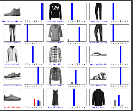
plt.show()# Plot the first X test images, their predicted labels, and the true labels.
# Color correct predictions in blue and incorrect predictions in red.
num_rows = 5
num_cols = 3
num_images = num_rows * num_cols
plt.figure(figsize=(2 * 2 * num_cols, 2 * num_rows))
for i in range(num_images):plt.subplot(num_rows, 2 * num_cols, 2 * i + 1)plot_image(i, predictions[i], test_labels, test_images)plt.subplot(num_rows, 2 * num_cols, 2 * i + 2)plot_value_array(i, predictions[i], test_labels)
plt.tight_layout()
plt.show()# Grab an image from the test dataset.
img = test_images[1]print(img.shape)# Add the image to a batch where it's the only member.
img = (np.expand_dims(img, 0))print(img.shape)predictions_single = probability_model.predict(img)print(predictions_single)plot_value_array(1, predictions_single[0], test_labels)
_ = plt.xticks(range(10), class_names, rotation=45)
plt.show()print(np.argmax(predictions_single[0]))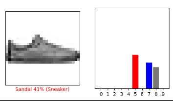
这篇关于Basic classification: Classify images of clothing的文章就介绍到这儿,希望我们推荐的文章对编程师们有所帮助!

