【RL】Basic Concepts in Reinforcement Learning

本文主要是介绍【RL】Basic Concepts in Reinforcement Learning，希望对大家解决编程问题提供一定的参考价值，需要的开发者们随着小编来一起学习吧！

Lecture1: Basic Concepts in Reinforcement Learning

MDP(Markov Decision Process)

Key Elements of MDP

Set

State: The set of states $\mathcal{S}$（状态$\mathcal{S}$的集合）

Action: the set of actions $\mathcal{A}(s)$ is associated for state $s\in \mathcal{S}$（对应于状态$s\in \mathcal{S}$ 的行为集合 $\mathcal{A}(s)$）

Reward: the set of rewards $\mathcal{R}(s,a)$（对应于某一状态$s\in \mathcal{S}$ 和在该状态的某一行为$a\in \mathcal{A}(s)$的奖励分数，是一个实数）

Probability distribution

State transition probability: at state $s$ ,taking action $a$, the probability to transit to state $s^{\prime }$ is （状态转移概率，在状态$s$，行为$a$，转移到状态$s^{\prime }$的概率）
$$p(s^{\prime }|s,a)$$
Reward probability: at state $s$, taking action $a$, the probability to get reward $r$ is （在状态$s$，行为$a$，得到的奖励分数$r$）
$$p(r|s,a)$$

Policy

Policy: at state $s$, the probability to choose action $a$ is（在状态$s\in \mathcal{S}$，选择状态$a\in \mathcal{A}(s)$的概率）
$$\pi (a|s)$$

Markov Property

Markov property: memoryless property （无记忆性；无后效性）
$$\begin{gathered} p(s_{t+1}|a_{t+1},s_t,...,a_1,s_0)=p(s_{t+1}|a_{t+1},s_t) \\ p(r_{t+1}|a_{t+1},s_t,...,a_1,s_0)=p(r_{t+1}|a_{t+1},s_t) \end{gathered}$$

Grid-World Example

以grid-world为例对上面例子进行解释

Key Elements

state： 每个表格所在的位置即为state, 因此其有9个state $s_1,s_2,...,s_9$。

每个表格所在的位置即为state, 因此其有9个state $s_1,s_2,...,s_9$。

state space： S = { s i } i = 1 9 \mathcal{S} = \{ s_i \}^9_{i=1} S={si​}i=19​

action：对于每一个state，有五个可能的action

• $a_1$: move upwards
• $a_2$: move rightwards
• $a_3$: move downwards
• $a_4$: move leftwards
• $a_5$: stay unchanged

Action space of a state：特定state其所有可能的action的集合 A ( s ) = { a i } i = 1 5 \mathcal{A}(s)= \{ a_i \}^5_{i=1} A(s)={ai​}i=15​

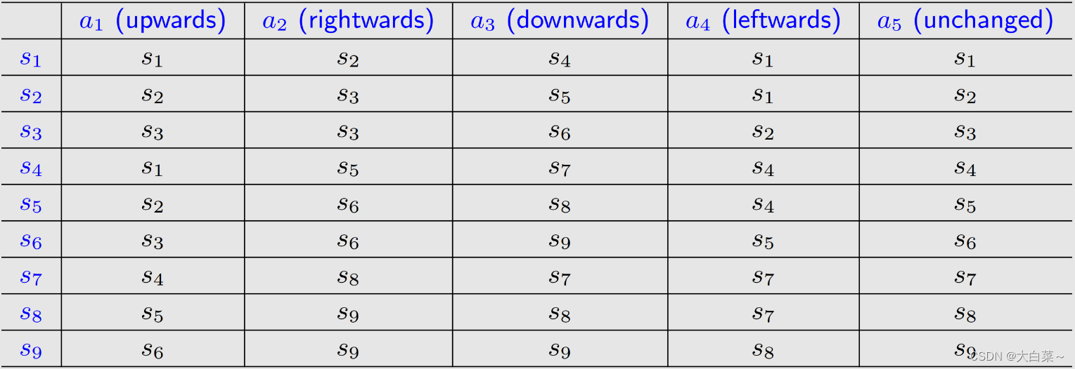
state transition

当采取action时，agent可能会从一个state转移到另一个state。例如 $s_1\stackrel{a_2}{⟶}{s}_1$

• tubular representation: 使用表格表示state transition

  

• state transition probability: 使用概率描述state transition

  • intuition: 在state $s_1$，如果选择action$a_2$，下一个state是$s_2$

  • math:
    $$\begin{array}{rl}& p(s_2|s_1,a_2)=1\\ & p(s_i|s_1,a_2)=0\forall \ne 2\end{array}$$

Policy

告诉agent在某个state下要采取什么action。

直观表示如下图所示：

基于以上policy，针对不同的start area和end area，最优路径如下：

mathematical representation: 使用条件概率表示
$$\begin{gathered} \pi (a_1|s_1)=0 \\ \pi (a_2|s_1)=1 \\ \pi (a_3|s_1)=0 \\ \pi (a_4|s_1)=0 \\ \pi (a_5|s_1)=0 \end{gathered}$$
其上为确定概率，也有随机概率：

$$\begin{array}{rl}& \pi (a_1|s_1)=0\\ & \pi (a_2|s_1)=0.5\\ & \pi (a_3|s_1)=0.5\\ & \pi (a_4|s_1)=0\\ & \pi (a_5|s_1)=0\end{array}$$
tabular representation: 使用表格表示

Reward

在采取某个action后得到的实数

• 正数代表鼓励去采取这种action
• 复数代表惩罚采取这种action
• 零代表不鼓励不惩罚

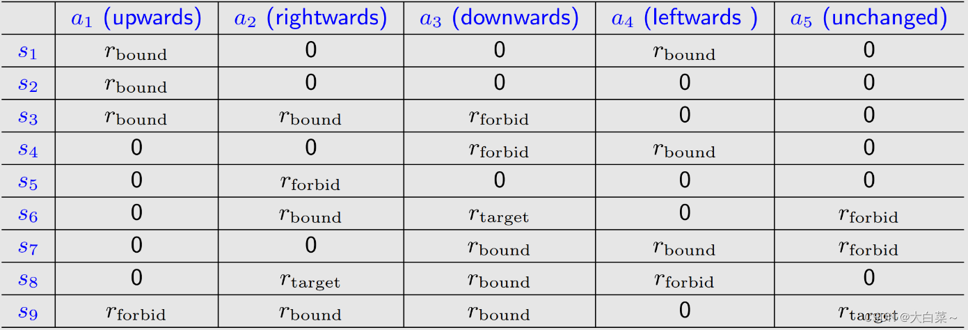
对于grid-world样例，reward可以设计成以下四种：

• 如果agent尝试逃出表格边界：$r_{round}=-1$
• 如果agent尝试进入禁区（蓝色方块）：$r_{forbid}=-1$
• 如果agent到达目标单元：$r_{target}=1$
• 其他情况：$r=0$

reward可以理解为human-machine interface，通过它我们可以引导agent按照我们的期望行事。

• tabular representation:

  

• Mathematical description:
  $$\begin{gathered} p(r=-1|s_1,a_1)=1 \\ p(r\ne -1|s_1,a_1)=0 \end{gathered}$$

Trajectory and Return

如下图：

trajectory 是一个state-action-reward 链：
$$s_1\underset{r=0}{\overset{a_2}{\to }}{s}_2\underset{r=0}{\overset{a_3}{\to }}{s}_5\underset{r=0}{\overset{a_3}{\to }}{s}_8\underset{r=1}{\overset{a_2}{\to }}{s}_9$$
return是沿该轨迹收集的所有奖励的总和：
$$\text{return}=0+0+0+1=1$$

Discounted return

对于下图trajectory ：

其可以定义为：
$$s_1\stackrel{a_2}{\to }{s}_2\stackrel{a_3}{\to }{s}_5\stackrel{a_3}{\to }{s}_8\stackrel{a_2}{\to }{s}_9\stackrel{a_5}{\to }{s}_9\stackrel{a_5}{\to }{s}_9...$$
return为：
$$\text{return}=0+0+0+1+1+1+...=\infty$$
需要引入discount rate $\gamma \in [0,1)$

discount return:
$$\begin{array}{rl}\text{discount return}& =0+\gamma 0+{\gamma }^{2}0+{\gamma }^{3}1+{\gamma }^{4}1+...\\ & ={\gamma }^3(1+\gamma +{\gamma }^2+...)\\ & ={\gamma }^3\frac{1}{1-\gamma }\end{array}$$

• 如果$\gamma$接近于0，则discounted return的值主要由近期获得的reward决定。
• 如果$\gamma$接近于1，则discounted return的值主要由远期获得的reward决定。

Episode

当遵循policy与环境交互时，agent可能会停在某些terminal states。 由此产生的轨迹称为一个episode（或一次trail）。

如上图，episode为:
$$s_1\underset{r=0}{\overset{a_2}{\to }}{s}_2\underset{r=0}{\overset{a_3}{\to }}{s}_5\underset{r=0}{\overset{a_3}{\to }}{s}_8\underset{r=1}{\overset{a_2}{\to }}{s}_9$$

一个episode通常被假设为一个有限的trajectory。 具有episodes的任务称为episodic tasks

有些任务可能没有终止状态（terminal states），这意味着与环境的交互永远不会结束。 此类任务称为连续任务（continuing tasks）

事实上，可以通过将episodic 任务转换为连续任务，以统一的数学方式来处理episodic任务和连续任务。

• 选择1：将目标状态视为特殊的吸收状态（absorbing state）。 一旦agent达到吸收状态，它就永远不会离开。 随之而来的奖励 $r=0$
• 选择2：将目标状态视为具有策略的正常状态。 agent仍然可以离开目标状态，并在进入目标状态时获得 $r=+1$。

选择2是较多人选择的方法。

Markov decision process (MDP)

grid-world可以抽象为一个更通用的模型，即马尔可夫过程。

圆圈代表state，带箭头的链接代表state transition。
一旦给出policy，马尔可夫决策过程就变成马尔可夫过程。



以上内容为B站西湖大学智能无人系统 强化学习的数学原理 公开课笔记。

这篇关于【RL】Basic Concepts in Reinforcement Learning的文章就介绍到这儿，希望我们推荐的文章对编程师们有所帮助！

---