【机器学习实战】二、随机森林算法预测出租车车费案例

随机森林算法预测出租车车费案例

一、导入第三方库

import numpy as np
import pandas as pd
import matplotlib.pyplot as plt
import seaborn as sns
import sklearn

二、加载数据集

train = pd.read_csv('train.csv',nrows=1000000) # 加载前1000000条数据
test = pd.read_csv('test.csv')

三、数据分析、清洗

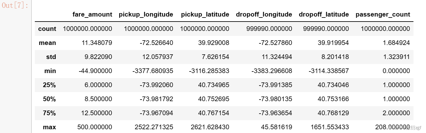
train.shape # 训练集的形状
# 输出：(1000000,8)

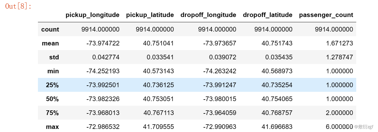
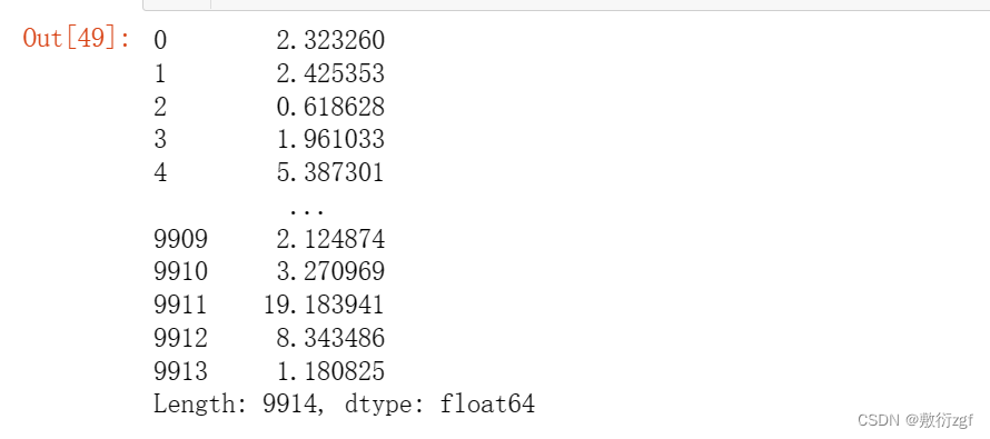
test.shape # 测试集的形状
# 输出：(9914, 7)

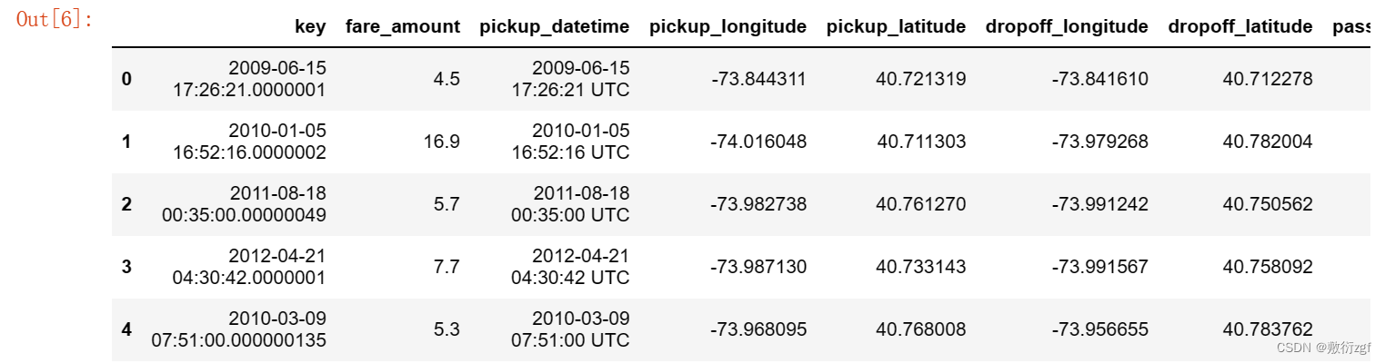
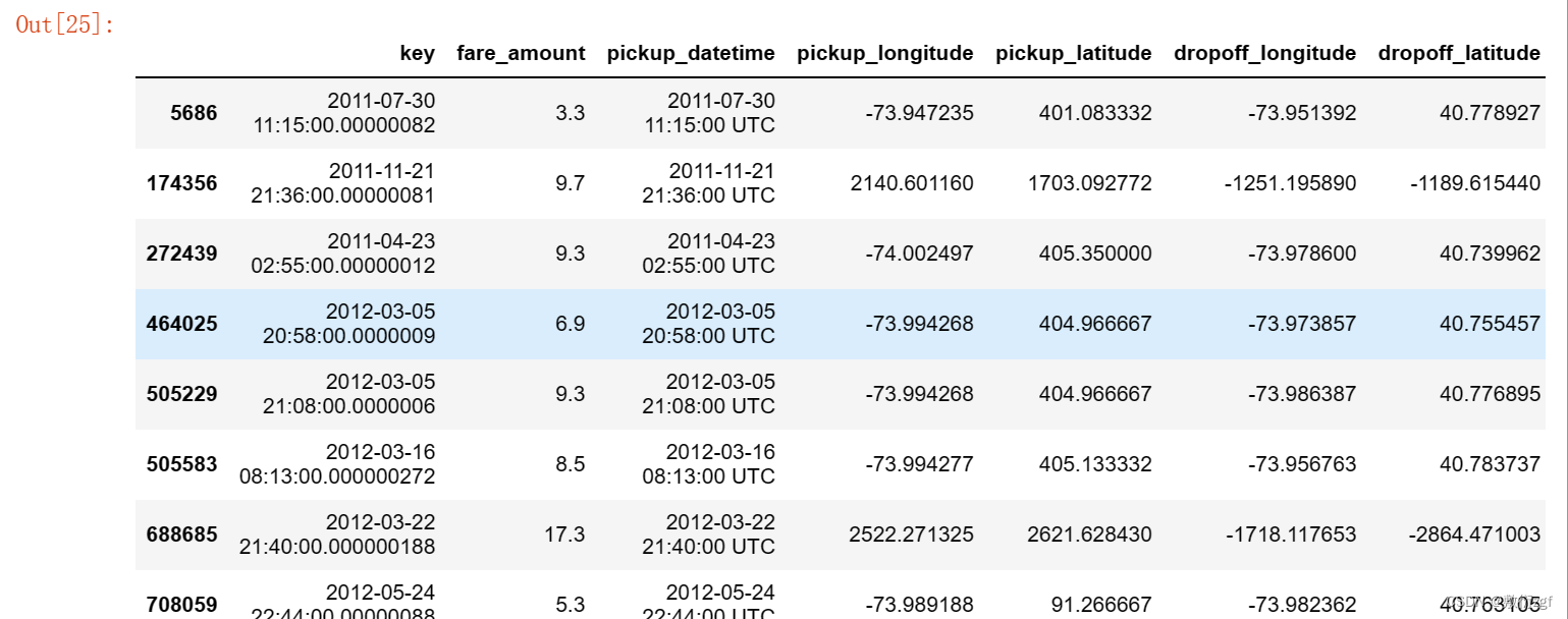
train.head() # 显示训练集的前五行数据

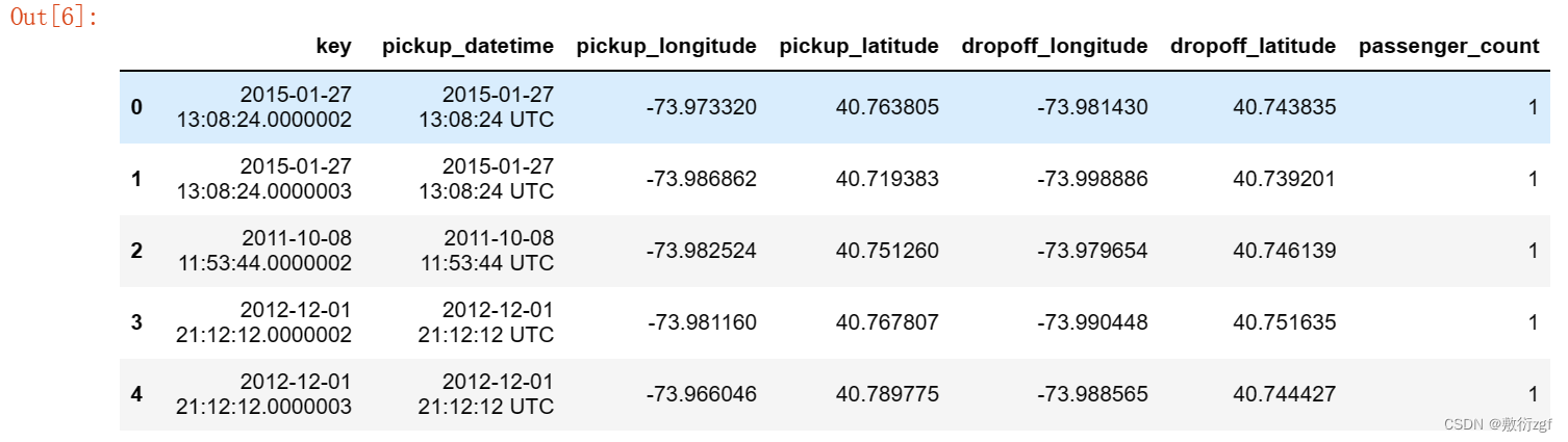
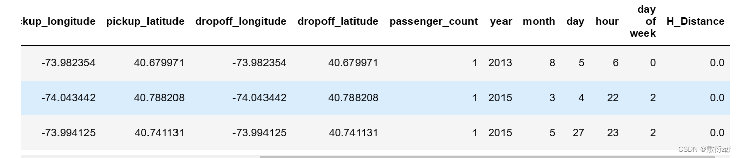
test.head() # 显示前5行测试集数据

train.describe() # 描述训练集

test.describe() # 描述测试集

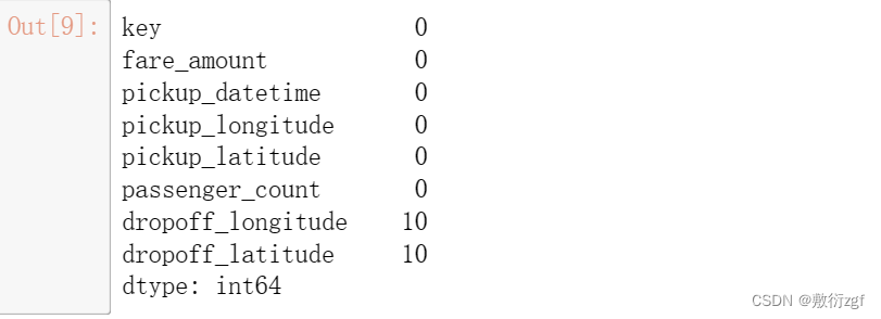
（1）检查数据中是否有空值

train.isnull().sum().sort_values(ascending=True) # 统计空值的数量，根据数量大小排序

test.isnull().sum().sort_values(ascending=True) #  统计空值数量

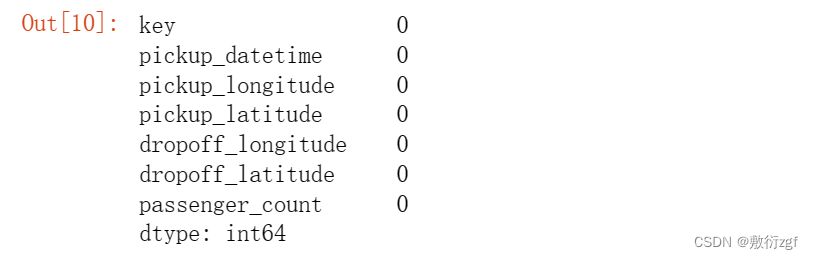
# 删除train中的空值
train.drop(train[train.isnull().any(1)].index, axis=0,inplace=True)
train.shape # 比原始数据减少10行
# 输出 (999990,8)

（2）检查fare_amount列是否有不合法值

train['fare_amount'].describe() # 描述fare_amount

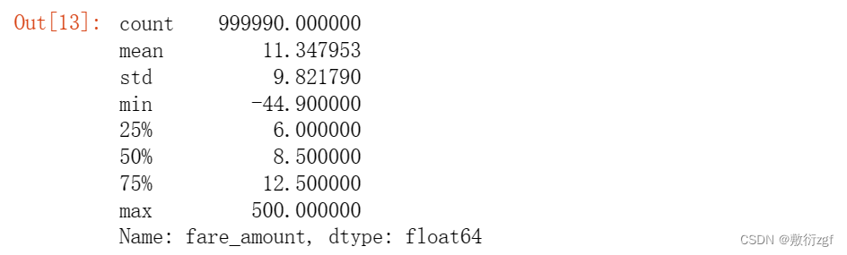
# 将fare_amount的值小于0的进行统计
from collections import Counter
Counter(train['fare_amount'] < 0 ) # 共计38行车费小于0的数据
# 输出：Counter({False: 999952, True: 38})

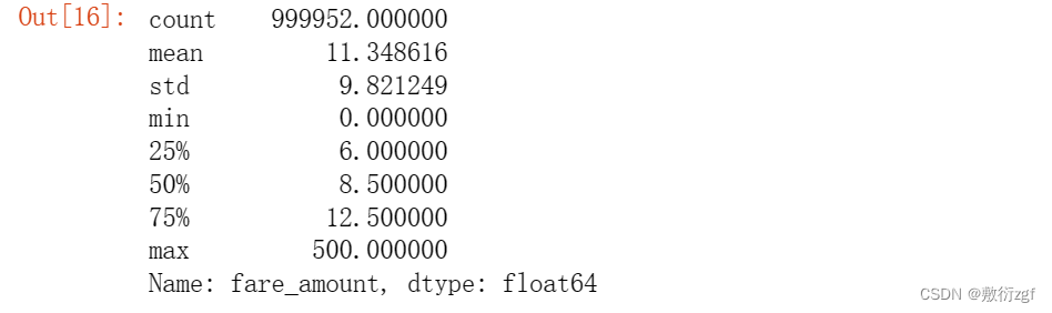
# 将这38行数据删除
train.drop(train[train['fare_amount']<0].index,axis=0,inplace=True)
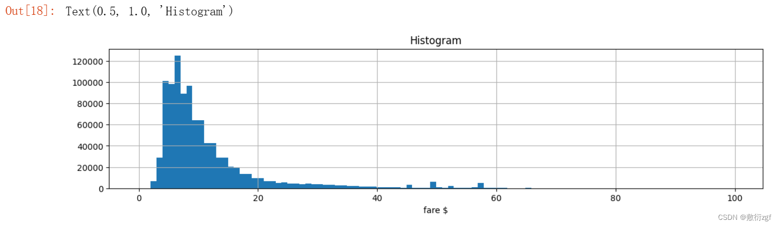
train['fare_amount'].describe()# 查看车费数据

# 可视化（直方图）：0<票价<100   bins=100 划分为100份 
train[train.fare_amount<100].fare_amount.hist(bins=100,figsize=(14,3)) 
plt.xlabel('fare $')
plt.title('Histogram')

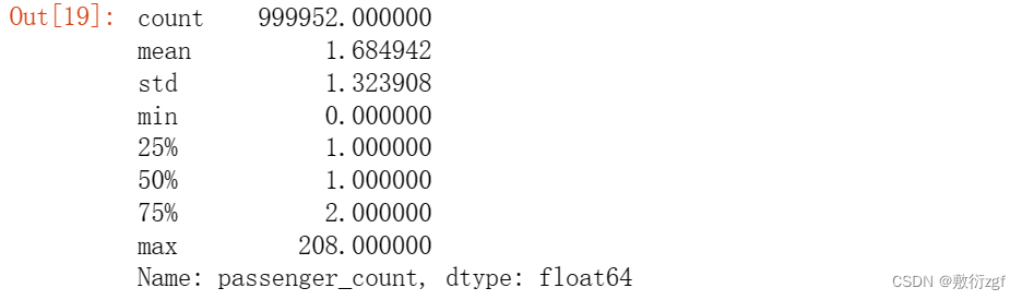
(3) 检查乘客passenger_count这一列

train['passenger_count'].describe() # 描述passenger_count这一列

# 查看乘客人数大于6的数据
train[train['passenger_count']>6]

# 删除离异值
train.drop(train[train['passenger_count']>6].index,axis=0,inplace=True)

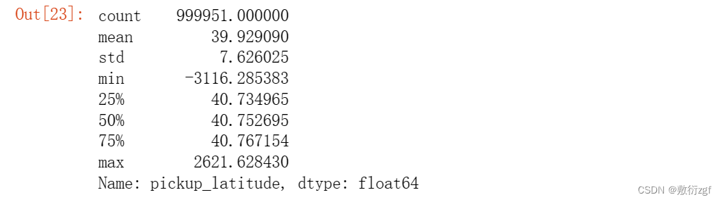
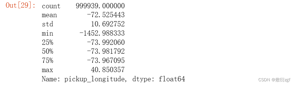
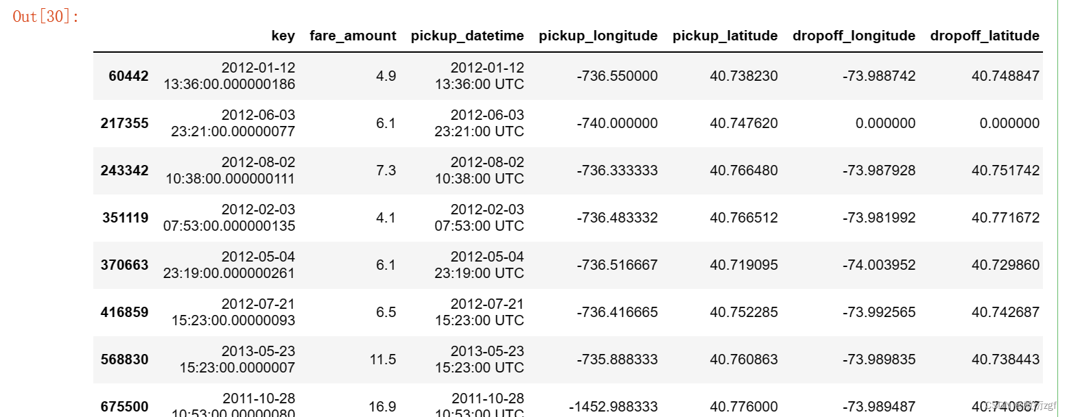
(4)检查上车点的经度和纬度
1.纬度范围：-90 ~ 90
2.经度范围：-180 ~ 180

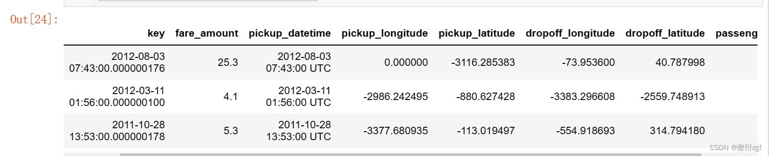
train['pickup_latitude'].describe() # 查看上车点纬度数据（min和max的离异值）

# 查看纬度小于 -90 的数据
train[train['pickup_latitude']< -90]

# 查看纬度大于 90 的数据
train[train['pickup_latitude'] > 90]

# 删除离异值
train.drop(train[(train['pickup_latitude'] > 90) | (train['pickup_latitude'] < -90 )].index, axis= 0 , inplace = True)

train.shape
# 输出：(999939, 8)

train['pickup_longitude'].describe() # 查看上车点的经度数据

train[train['pickup_longitude'] < - 180]

# 删除这些数据
train.drop(train[train['pickup_longitude'] < -180 ].index , axis=0 , inplace =True)
train.shape
# 输出：(999928, 8)

（5）检查下车点的经度和纬度

train.drop(train[(train['dropoff_latitude'] < -90 ) | (train['dropoff_latitude'] > 90 )].index, axis=0,inplace=True)

train.drop(train[(train['dropoff_longitude'] < -180 )| (train['dropoff_longitude'] > 180 )].index, axis=0 ,inplace= True)
train.shape
# 输出：(999911, 8)

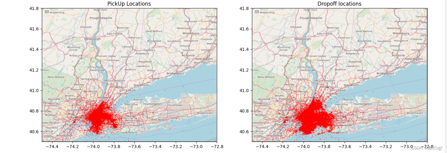
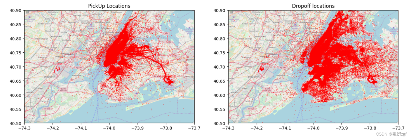
（6）可视化地图，清理一些离异值

# 在测试集上确定一个区域，删除掉train数据集中不在区域框内的奇异点
# （1）纬度最小值，纬度最大值
min(test.pickup_latitude.min(),test.dropoff_latitude.min()), \
max(test.pickup_latitude.max(),test.dropoff_latitude.max())
# 输出： (40.568973, 41.709555)

# （2）经度最小值，经度最大值
min(test.pickup_longitude.min(), test.dropoff_longitude.min()), \
max(test.pickup_longitude.max(), test.dropoff_longitude.max())
# 输出：(-74.263242, -72.986532)

# （3）根据指定的区域框，删除掉奇异点
def select_within_boundingbox(df,BB):return (df.pickup_longitude >= BB[0]) & (df.pickup_longitude <= BB[1]) & \(df.pickup_latitude >= BB[2]) & (df.pickup_latitude <= BB[3]) & \(df.dropoff_longitude >= BB[0]) & (df.dropoff_longitude <= BB[1]) & \(df.dropoff_latitude >= BB[2]) & (df.dropoff_latitude <= BB[3])

BB = (-74.5,-72.8,40.5,41.8)
# 截图
nyc_map = plt.imread('./nyc_-74.5_-72.8_40.5_41.8.png')

BB_zoom = (-74.3, -73.7, 40.5, 40.9) # 放大后的地图
# 截图（放大）
nyc_map_zoom = plt.imread('./nyc_-74.3_-73.7_40.5_40.9.png')

train = train[select_within_boundingbox(train, BB)]# 删除区域框之外的点

train.shape
# 输出：(979018, 8)

# （4）在地图显示这些点def plot_on_map(df, BB, nyc_map, s=10, alpha=0.2):fig, axs = plt.subplots(1, 2, figsize=(16,10))# 第一个子图axs[0].scatter(df.pickup_longitude, df.pickup_latitude, alpha=alpha, c='r', s=s)axs[0].set_xlim(BB[0], BB[1])axs[0].set_ylim(BB[2], BB[3])axs[0].set_title('PickUp Locations')axs[0].imshow(nyc_map, extent=BB)# 第二个子图axs[1].scatter(df.dropoff_longitude, df.dropoff_latitude, alpha=alpha, c='r', s=s)axs[1].set_xlim((BB[0], BB[1]))axs[1].set_ylim((BB[2], BB[3]))axs[1].set_title('Dropoff locations')axs[1].imshow(nyc_map, extent=BB)

plot_on_map(train, BB, nyc_map, s=1, alpha=0.3)

plot_on_map(train, BB_zoom, nyc_map_zoom, s=1, alpha=0.3)

(7) 检查数据类型

train.dtypes

# 日期类型转换：key, pickup_datetimefor dataset in [train, test]:dataset['key'] = pd.to_datetime(dataset['key'])dataset['pickup_datetime'] = pd.to_datetime(dataset['pickup_datetime'])

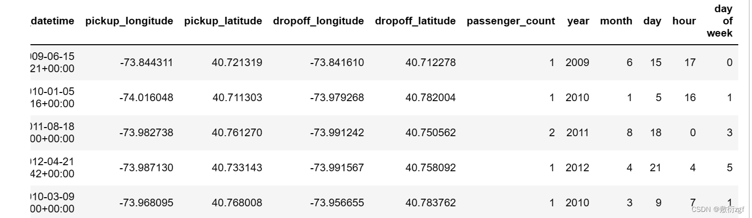
（8）日期数据进行分析
将日期分隔为： 1.year 2.month 3.day 4.hour 5.day of week

# 增加5列，分别是：year, month, day, hour, day of weekfor dataset in [train, test]:dataset['year'] = dataset['pickup_datetime'].dt.yeardataset['month'] = dataset['pickup_datetime'].dt.monthdataset['day'] = dataset['pickup_datetime'].dt.daydataset['hour'] = dataset['pickup_datetime'].dt.hourdataset['day of week'] = dataset['pickup_datetime'].dt.dayofweek
train.head()

test.head()

（9）根据经纬度计算距离

# 计算公式def distance(lat1, long1, lat2, long2):data = [train, test]for i in data:R = 6371  # 地球半径（单位：千米）phi1 = np.radians(i[lat1])phi2 = np.radians(i[lat2])delta_phi = np.radians(i[lat2]-i[lat1])delta_lambda = np.radians(i[long2]-i[long1])#a = sin²((φB - φA)/2) + cos φA . cos φB . sin²((λB - λA)/2)a = np.sin(delta_phi / 2.0) ** 2 + np.cos(phi1) * np.cos(phi2) * np.sin(delta_lambda / 2.0) ** 2#c = 2 * atan2( √a, √(1−a) )c = 2 * np.arctan2(np.sqrt(a), np.sqrt(1-a))#d = R*cd = (R * c) # 单位：千米i['H_Distance'] = dreturn d

distance('pickup_latitude','pickup_longitude','dropoff_latitude','dropoff_longitude')

# 统计距离为0，票价为0的数据train[(train['H_Distance']==0) & (train['fare_amount']==0)]

# 删除
train.drop(train[(train['H_Distance']==0) & (train['fare_amount']==0)].index, axis=0, inplace=True)

# 统计距离为0，票价不为0的数据# 原因1：司机等待乘客很长时间，乘客最终取消了订单，乘客依然支付了等待的费用；
# 原因2：车辆的经纬度没有被准确录入或缺失；len(train[(train['H_Distance']==0) & (train['fare_amount']!=0)])
# 输出：10478

# 删除
train.drop(train[(train['H_Distance']==0) & (train['fare_amount']!=0)].index, axis=0, inplace=True)

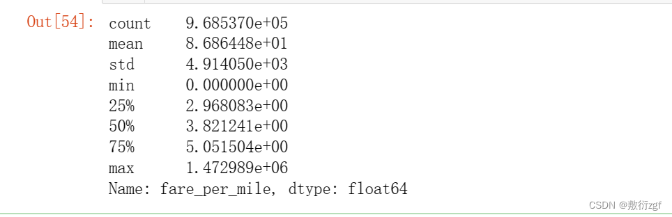
（10）新的字段：每公里车费：根据距离、车费，计算每公里的车费

train['fare_per_mile'] = train.fare_amount / train.H_Distancetrain.fare_per_mile.describe()

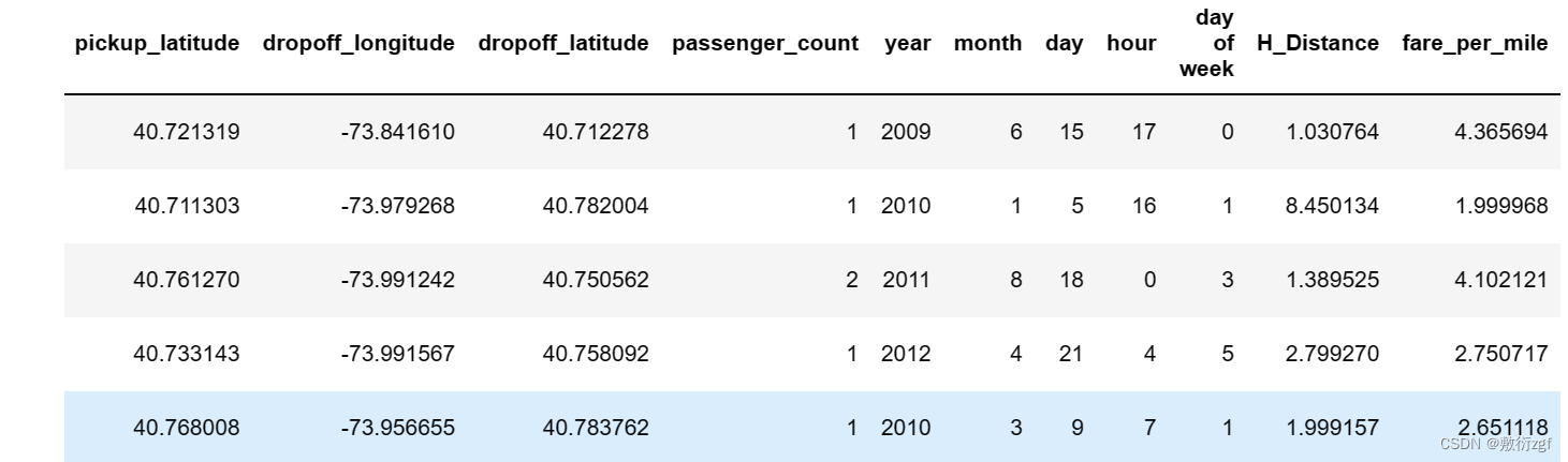
train.head()

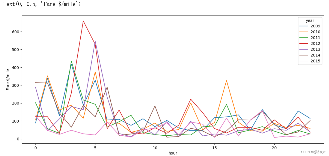
# 统计每一年的不同时间段的每小时车费train.pivot_table('fare_per_mile', index='hour', columns='year').plot(figsize=(14, 6))
plt.ylabel('Fare $/mile')

四、模型训练和数据预测

train.columns

test.columns

X_train = train.iloc[:,[3,4,5,6,7,8,9,10,11,12,13]]
y_train = train.iloc[:,[1]] # fare_amount 车费
X_train.shape
# 输出：(968537, 11)
y_train.shape
# 输出：(968537, 1)

五、随机森林算法实现

from sklearn.ensemble import RandomForestRegressor
rf = RandomForestRegressor()
rf.fit(X_train,y_train)

test.columns

rf_predict = rf.predict(test.iloc[:, [2,3,4,5,6,7,8,9,10,11,12]])

submission = pd.read_csv("sample_submission.csv")submission.head()

# 提交submission = pd.read_csv("sample_submission.csv")submission['fare_amount'] = rf_predictsubmission.to_csv("submission_1.csv", index=False)submission.head()