PaddleHub - 波士顿房价预测

背景

经典的线性回归模型主要用来预测一些存在着线性关系的数据集。回归模型可以理解为：存在一个点集，用一条曲线去拟合它分布的过程。如果拟合曲线是一条直线，则称为线性回归。如果是一条二次曲线，则被称为二次回归。线性回归是回归模型中最简单的一种。 本教程使用PaddlePaddle建立起一个房价预测模型。

在线性回归中：
（1）假设函数是指，用数学的方法描述自变量和因变量之间的关系，它们之间可以是一个线性函数或非线性函数。 在本次线性回顾模型中，我们的假设函数为 Y’= wX+b ，其中，Y’表示模型的预测结果（预测房价），用来和真实的Y区分。模型要学习的参数即：w,b。

（2）损失函数是指，用数学的方法衡量假设函数预测结果与真实值之间的误差。这个差距越小预测越准确，而算法的任务就是使这个差距越来越小。 建立模型后，我们需要给模型一个优化目标，使得学到的参数能够让预测值Y’尽可能地接近真实值Y。这个实值通常用来反映模型误差的大小。不同问题场景下采用不同的损失函数。 对于线性模型来讲，最常用的损失函数就是均方误差（Mean Squared Error， MSE）。

（3）优化算法：神经网络的训练就是调整权重（参数）使得损失函数值尽可能得小，在训练过程中，将损失函数值逐渐收敛，得到一组使得神经网络拟合真实模型的权重（参数）。所以，优化算法的最终目标是找到损失函数的最小值。而这个寻找过程就是不断地微调变量w和b的值，一步一步地试出这个最小值。 常见的优化算法有随机梯度下降法（SGD）、Adam算法等等

首先导入必要的包

paddle.fluid—>PaddlePaddle深度学习框架
numpy---------->python基本库，用于科学计算
os------------------>python的模块，可使用该模块对操作系统进行操作
matplotlib----->python绘图库，可方便绘制折线图、散点图等图形

import paddle.fluid as fluid
import paddle
import numpy as np
import os
import matplotlib.pyplot as plt

准备数据

uci-housing数据集介绍

数据集共506行,每行14列。前13列用来描述房屋的各种信息，最后一列为该类房屋价格中位数。
PaddlePaddle提供了读取uci_housing训练集和测试集的接口，分别为paddle.dataset.uci_housing.train()和paddle.dataset.uci_housing.test()。

train_reader和test_reader

paddle.reader.shuffle()表示每次缓存BUF_SIZE个数据项，并进行打乱
paddle.batch()表示每BATCH_SIZE组成一个batch

BUF_SIZE=500
BATCH_SIZE=20#用于训练的数据提供器，每次从缓存中随机读取批次大小的数据
train_reader = paddle.batch(paddle.reader.shuffle(paddle.dataset.uci_housing.train(), buf_size=BUF_SIZE),                    batch_size=BATCH_SIZE)   
#用于测试的数据提供器，每次从缓存中随机读取批次大小的数据
test_reader = paddle.batch(paddle.reader.shuffle(paddle.dataset.uci_housing.test(),buf_size=BUF_SIZE),batch_size=BATCH_SIZE)  

网络配置

网络搭建

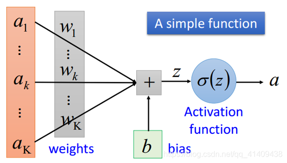
对于线性回归来讲，它就是一个从输入到输出的简单的全连接层。
对于波士顿房价数据集，假设属性和房价之间的关系可以被属性间的线性组合描述。

#定义张量变量x，表示13维的特征值
x = fluid.layers.data(name='x', shape=[13], dtype='float32')
#定义张量y,表示目标值
y = fluid.layers.data(name='y', shape=[1], dtype='float32')
#定义一个简单的线性网络,连接输入和输出的全连接层
#input:输入tensor;
#size:该层输出单元的数目
#act:激活函数
y_predict=fluid.layers.fc(input=x,size=1,act=None)

定义损失函数

此处使用均方差损失函数。
square_error_cost(input,lable): 接受输入预测值和目标值，并返回方差估计,即为（y-y_predict）的平方

cost = fluid.layers.square_error_cost(input=y_predict, label=y) 
#求一个batch的损失值
avg_cost = fluid.layers.mean(cost)                              
#对损失值求平均值

定义优化函数

此处使用的是随机梯度下降。

optimizer = fluid.optimizer.SGDOptimizer(learning_rate=0.001)
opts = optimizer.minimize(avg_cost)
test_program = fluid.default_main_program().clone(for_test=True)

模型训练 and 模型评估

创建Executor

首先定义运算场所 fluid.CPUPlace()和 fluid.CUDAPlace(0)分别表示运算场所为CPU和GPU
Executor:接收传入的program，通过run()方法运行program。

use_cuda = False                         #use_cuda为False,表示运算场所为CPU;use_cuda为True,表示运算场所为GPU           
place = fluid.CUDAPlace(0) if use_cuda else fluid.CPUPlace()
exe = fluid.Executor(place)              #创建一个Executor实例exe
exe.run(fluid.default_startup_program()) #Executor的run()方法执行startup_program(),进行参数初始化

定义输入数据维度

DataFeeder负责将数据提供器（train_reader,test_reader）返回的数据转成一种特殊的数据结构，使其可以输入到Executor中。
feed_list设置向模型输入的向变量表或者变量表名

# 定义输入数据维度
feeder = fluid.DataFeeder(place=place, feed_list=[x, y])#feed_list:向模型输入的变量表或变量表名

定义绘制训练过程的损失值变化趋势的方法draw_train_process

iter=0;
iters=[]
train_costs=[]
def draw_train_process(iters,train_costs):title="training cost"plt.title(title, fontsize=24)plt.xlabel("iter", fontsize=14)plt.ylabel("cost", fontsize=14)plt.plot(iters, train_costs,color='red',label='training cost') plt.grid()plt.show()```
## 训练并保存模型
Executor接收传入的program,并根据feed map(输入映射表)和fetch_list(结果获取表) 向program中添加feed operators(数据输入算子)和fetch operators（结果获取算子)。 feed map为该program提供输入数据。fetch_list提供program训练结束后用户预期的变量。注：enumerate() 函数用于将一个可遍历的数据对象(如列表、元组或字符串)组合为一个索引序列，同时列出数据和数据下标，```python
EPOCH_NUM=50
model_save_dir = "/home/aistudio/work/fit_a_line.inference.model"for pass_id in range(EPOCH_NUM):                                  #训练EPOCH_NUM轮# 开始训练并输出最后一个batch的损失值train_cost = 0for batch_id, data in enumerate(train_reader()):              #遍历train_reader迭代器train_cost = exe.run(program=fluid.default_main_program(),#运行主程序feed=feeder.feed(data),              #喂入一个batch的训练数据，根据feed_list和data提供的信息，将输入数据转成一种特殊的数据结构fetch_list=[avg_cost])    if batch_id % 40 == 0:print("Pass:%d, Cost:%0.5f" % (pass_id, train_cost[0][0]))    #打印最后一个batch的损失值iter=iter+BATCH_SIZEiters.append(iter)train_costs.append(train_cost[0][0])# 开始测试并输出最后一个batch的损失值test_cost = 0for batch_id, data in enumerate(test_reader()):               #遍历test_reader迭代器test_cost= exe.run(program=test_program, #运行测试chengfeed=feeder.feed(data),               #喂入一个batch的测试数据fetch_list=[avg_cost])                #fetch均方误差print('Test:%d, Cost:%0.5f' % (pass_id, test_cost[0][0]))     #打印最后一个batch的损失值#保存模型# 如果保存路径不存在就创建
if not os.path.exists(model_save_dir):os.makedirs(model_save_dir)
print ('save models to %s' % (model_save_dir))
#保存训练参数到指定路径中，构建一个专门用预测的program
fluid.io.save_inference_model(model_save_dir,   #保存推理model的路径['x'],            #推理（inference）需要 feed 的数据[y_predict],      #保存推理（inference）结果的 Variablesexe)              #exe 保存 inference model
draw_train_process(iters,train_costs)

模型预测

创建预测用的Executor

infer_exe = fluid.Executor(place)    #创建推测用的executor
inference_scope = fluid.core.Scope() #Scope指定作用域

可视化真实值与预测值方法定义

infer_results=[]
groud_truths=[]
#绘制真实值和预测值对比图
def draw_infer_result(groud_truths,infer_results):title='Boston'plt.title(title, fontsize=24)x = np.arange(1,20) y = xplt.plot(x, y)plt.xlabel('ground truth', fontsize=14)plt.ylabel('infer result', fontsize=14)plt.scatter(groud_truths, infer_results,color='green',label='training cost') plt.grid()plt.show()```
## 开始预测
通过fluid.io.load_inference_model，预测器会从params_dirname中读取已经训练好的模型，来对从未遇见过的数据进行预测。
```python
with fluid.scope_guard(inference_scope):#修改全局/默认作用域（scope）, 运行时中的所有变量都将分配给新的scope。#从指定目录中加载 推理model(inference model)[inference_program,                             #推理的programfeed_target_names,                             #需要在推理program中提供数据的变量名称fetch_targets] = fluid.io.load_inference_model(#fetch_targets: 推断结果model_save_dir, #model_save_dir:模型训练路径 infer_exe)      #infer_exe: 预测用executor#获取预测数据infer_reader = paddle.batch(paddle.dataset.uci_housing.test(),  #获取uci_housing的测试数据batch_size=200)                           #从测试数据中读取一个大小为200的batch数据#从test_reader中分割xtest_data = next(infer_reader())test_x = np.array([data[0] for data in test_data]).astype("float32")test_y= np.array([data[1] for data in test_data]).astype("float32")results = infer_exe.run(inference_program,                              #预测模型feed={feed_target_names[0]: np.array(test_x)},  #喂入要预测的x值fetch_list=fetch_targets)                       #得到推测结果 print("infer results: (House Price)")for idx, val in enumerate(results[0]):print("%d: %.2f" % (idx, val))infer_results.append(val)print("ground truth:")for idx, val in enumerate(test_y):print("%d: %.2f" % (idx, val))groud_truths.append(val)draw_infer_result(groud_truths,infer_results)