【TI毫米波雷达】IWR6843AOPEVM-G+DCA1000EVM的mmWave Studio数据读取、配置及避坑

【TI毫米波雷达】IWR6843AOPEVM-G+DCA1000EVM的mmWave Studio数据读取、配置及避坑

mmWave Studio

硬件方面连接好以后 就可以打开mmWave Studio了

环境

需要安装mmWave SDK
以及MATLAB runtime
是运行项目所需要的库，没装它项目会运行不了

ww2.mathworks.cn/products/compiler/matlab-runtime.html

最新版可能有bug
推荐下载安装MCR_R2015aSP1_win32_installer.exe

in.mathworks.com/supportfiles/downloads/R2015a/deployment_files/R2015aSP1/installers/win32/MCR_R2015aSP1_win32_installer.exe

配置

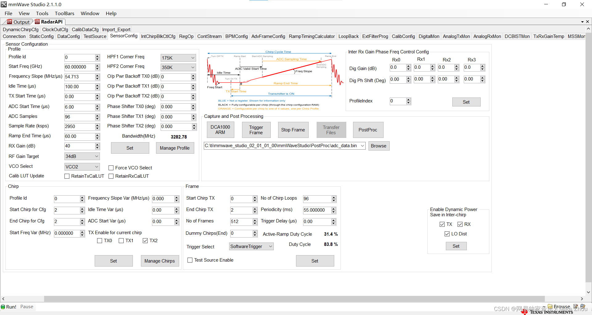
如果硬件配置成功 则可以通过mmWave Studio的Output看到配置信息

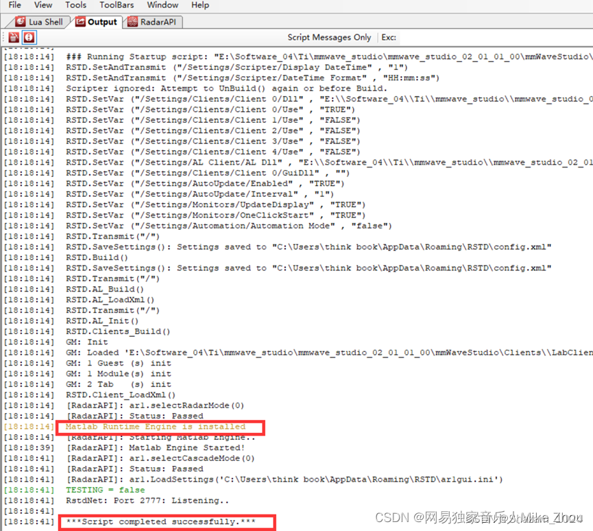
按照如图步骤 在radar api里面一步步来操作

Connection

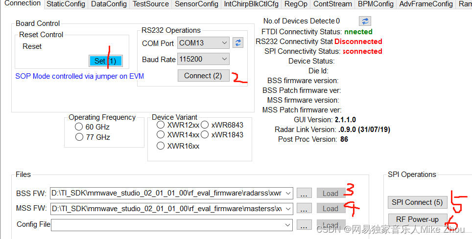
其中 RS232选择波特率115200 enhanced端口

BSS FW在路径：

D:\TI_SDK\mmwave_studio_02_01_01_00\rf_eval_firmware\radarss

MSS FW在：

D:\TI_SDK\mmwave_studio_02_01_01_00\rf_eval_firmware\masterss

选择好以后 点击加载
最后再点击SPI连接

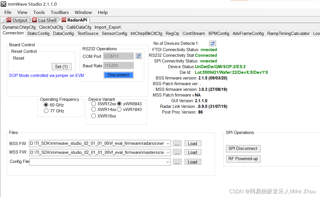
其中 雷达频率选择60GHz
连上以后：

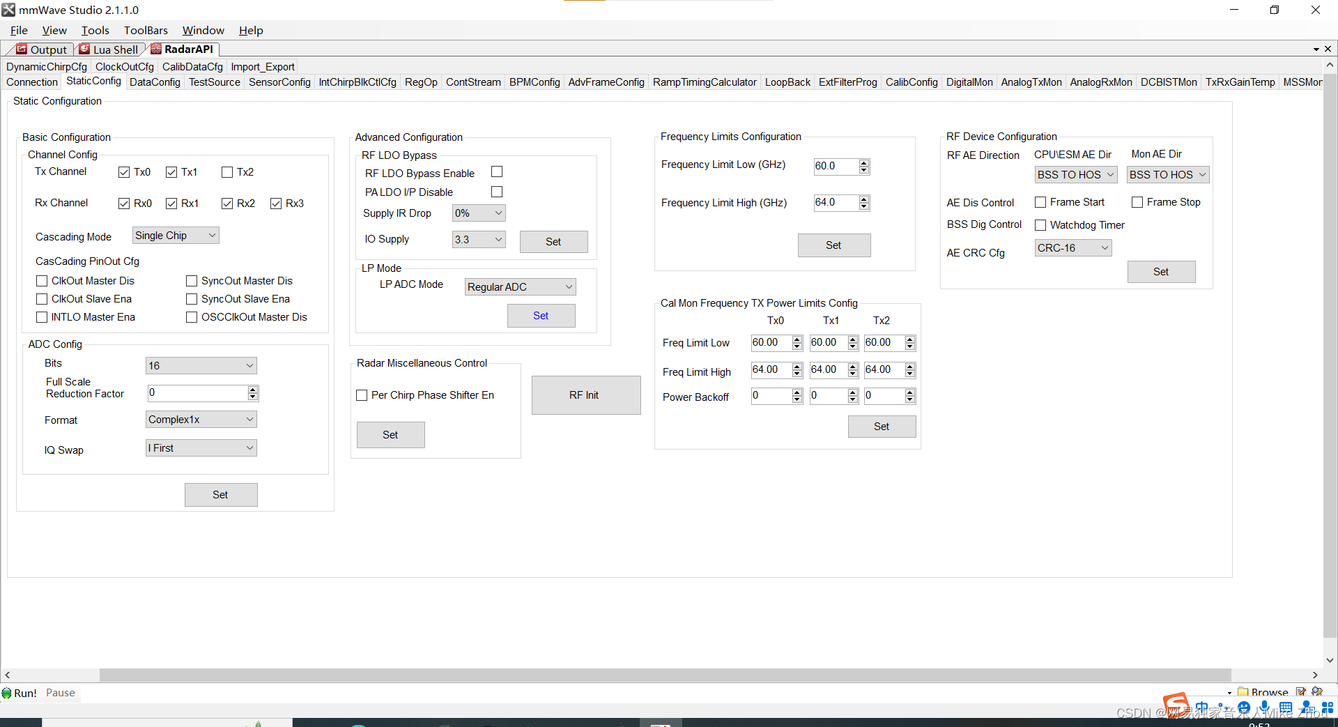
StaticCongfig

按照蓝色按钮标记，根据自己需求 更改参数配置，并一一点击set按钮配置。

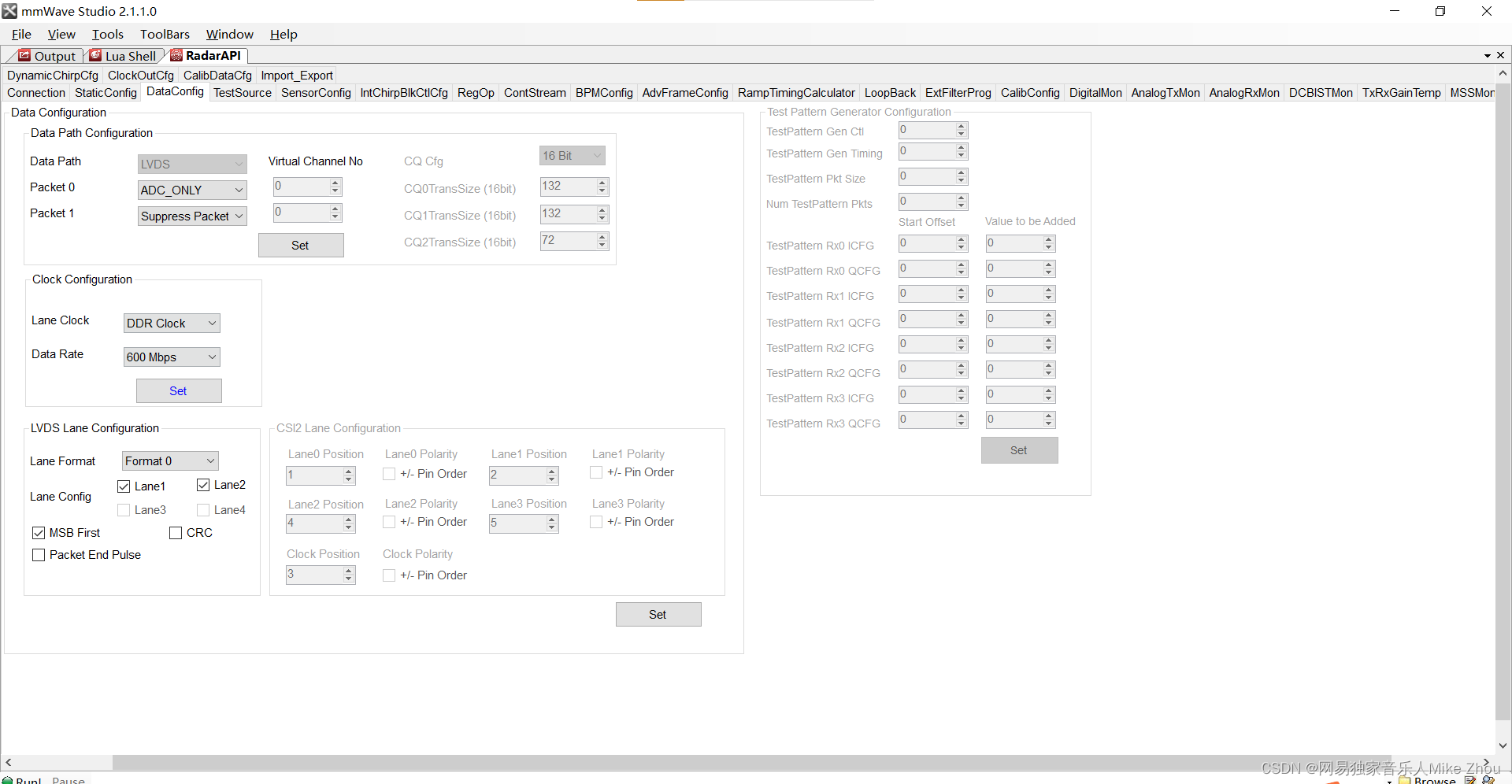
DataConfig

SensorConfig

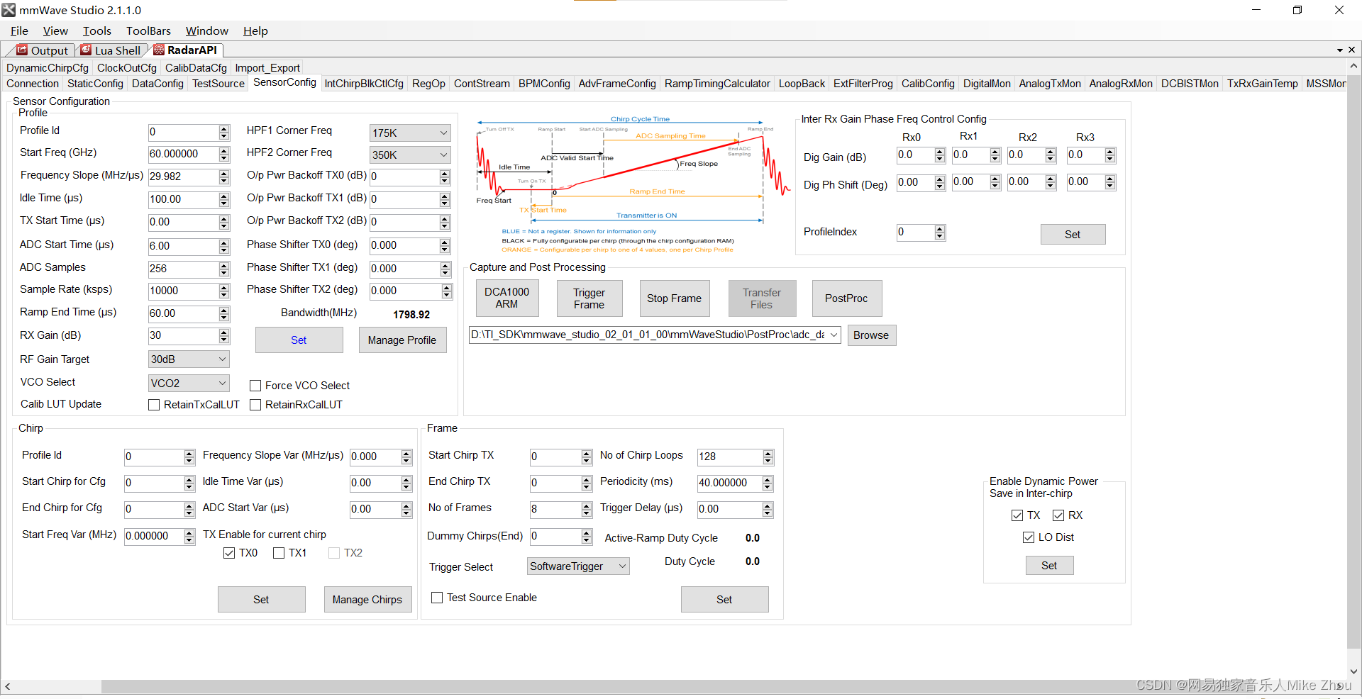
按提示配置完参数后即可开始采集。
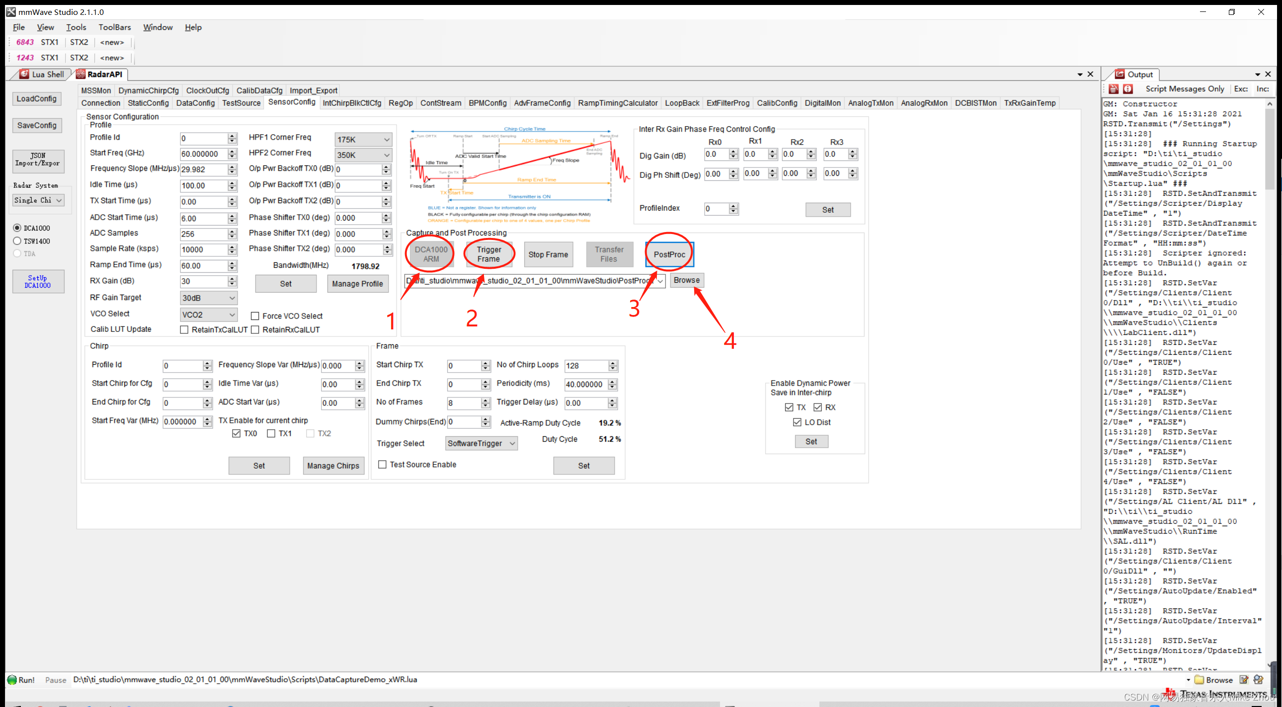
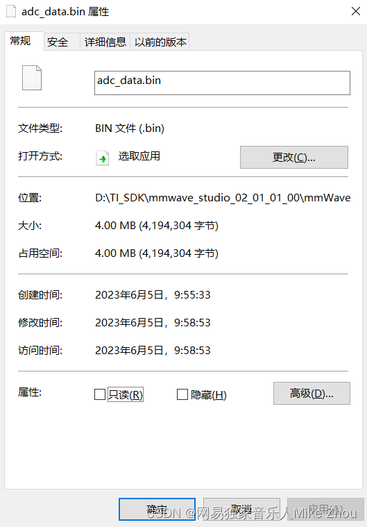
首先点击1️⃣DCA1000ARM，其实点击2️⃣Trigger Frame 便开始对雷达数据进行采集，最后采集完成，点击3️⃣PostProc便可查看雷达的数据处理后的效果图。采集到的原始数据存在4️⃣adc_data.bin文件中。
若没有数据产生 则肯定是没有连接到DCA1000ARM 需要点击左侧的SetUp DCA1000进行连接 同时 防火墙权限开到最大 或者干脆关闭防火墙

在进行第一步后 建议等待两秒再开始采集
tirrger frame就是开始采集 stop frame就是停止采集
生成的bin文件大小由配置决定 但数据由采集场景和时间等决定

雷达数据：

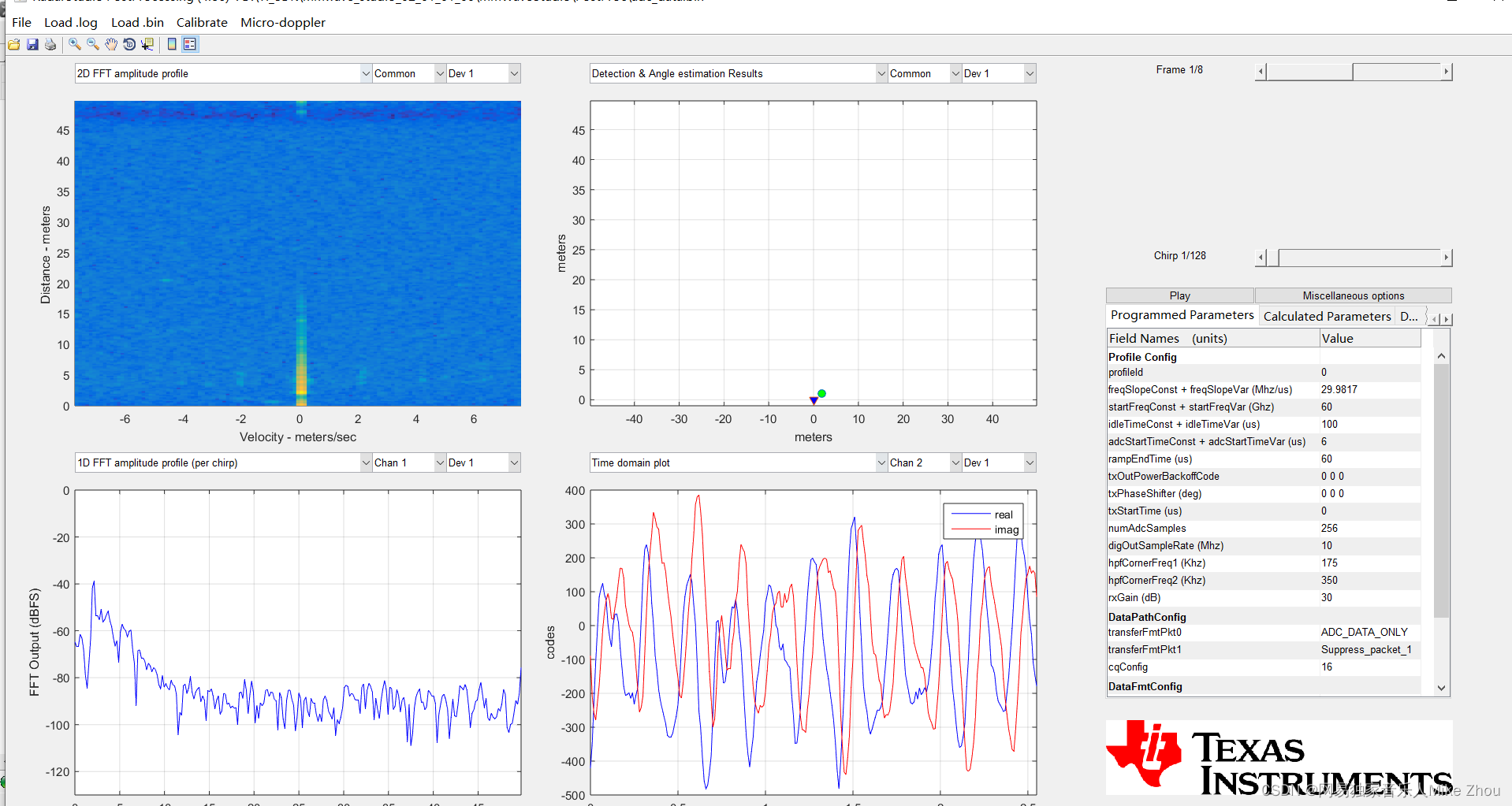
生成的数据：

报错解决方案

连接DCA1000时 Output报错 无法读取FPGA版本号等数据

Timeout Error! System disconnected

这是在连接FPGA时报错 网口的问题 防火墙设置为专用和公用网络都运行
或者IP没配置好
或者直接关闭防火墙
或者换个网口

连接SPI时报错 Output报错

MSS Power Up async event was not received!

检查DCA1000供电
将板子用UniFlash擦除后重连
或板子没有将开关设置为SPI模式 设置一下

附录：结构框架

雷达基本原理叙述

雷达工作原理是上电-发送chirps-帧结束-处理-上电循环
一个Frame，首先是信号发送，比如96个chirp就顺次发出去，然后接收回来，混频滤波，ADC采样，这些都是射频模块的东西。射频完成之后，FFT，CFAR，DOA这些就是信号处理的东西。然后输出给那个结构体，就是当前帧获得的点云了。

在射频发送阶段 一个frame发送若干个chirp 也就是上图左上角
第一个绿色点为frame start 第二个绿色点为frame end
其中发送若干chirps（小三角形）
chirps的个数称为numLoops（代码中 rlFrameCfg_t结构体）
在mmwave studio上位机中 则称为 no of chirp loops

frame end 到 周期结束的时间为计算时间 称为inter frame period

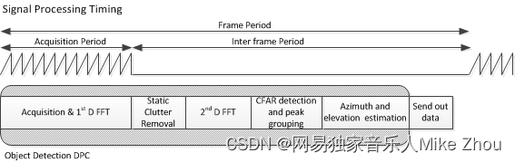
frame start到循环结束的时间称为framePeriodicity（代码中 rlFrameCfg_t结构体）
在mmwave studio上位机中 则称为 Periodicity

如下图frame配置部分

在inter frame Periodicity时间内（比如这里整个周期是55ms）
就是用于计算和处理的时间 一定比55ms要小
如果chirps很多的话 那么计算时间就会减小

如果是处理点云数据 则只需要每一帧计算一次点云即可
计算出当前帧的xyz坐标和速度 以及保存时间戳

雷达天线排列位置

在工业雷达包：

C:\ti\mmwave_industrial_toolbox_4_12_0\antennas\ant_rad_patterns

路径下 有各个EVM开发板的天线排列说明
同样的 EVM手册中也有
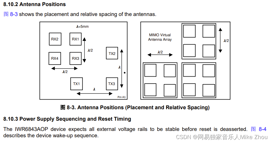
如IWR6843AOPEVM：


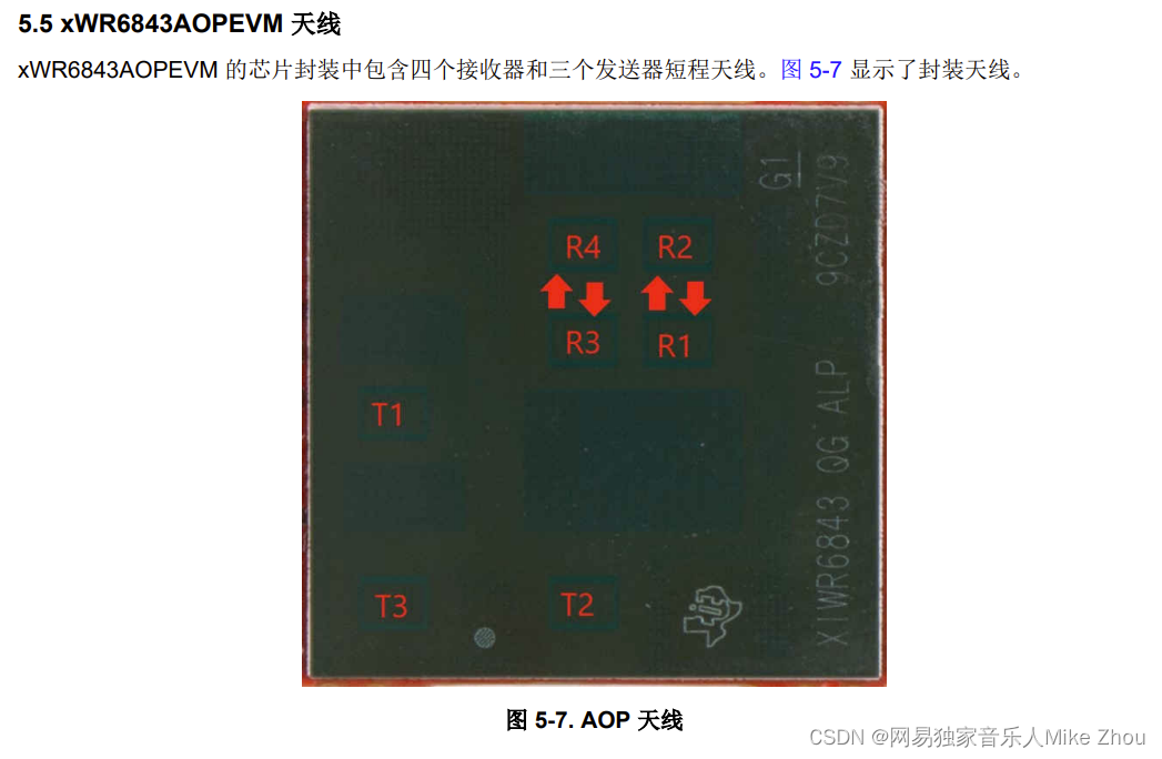
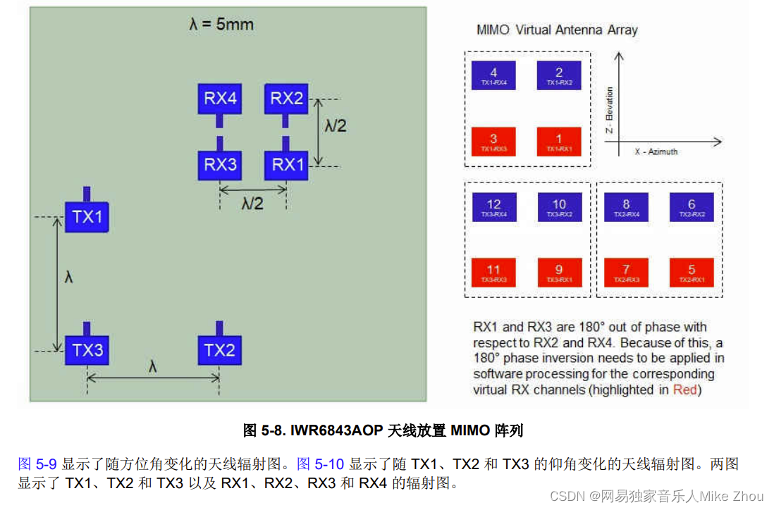
其天线的间距等等位于数据手册：

芯片框架

IWR6843AOP可以分成三个主要部分及多个外设
BSS：雷达前端部分
MSS：cortex-rf4内核 主要用于控制
DSS： DSP C674内核 主要用于信号处理
外设：UART GPIO DPM HWA等

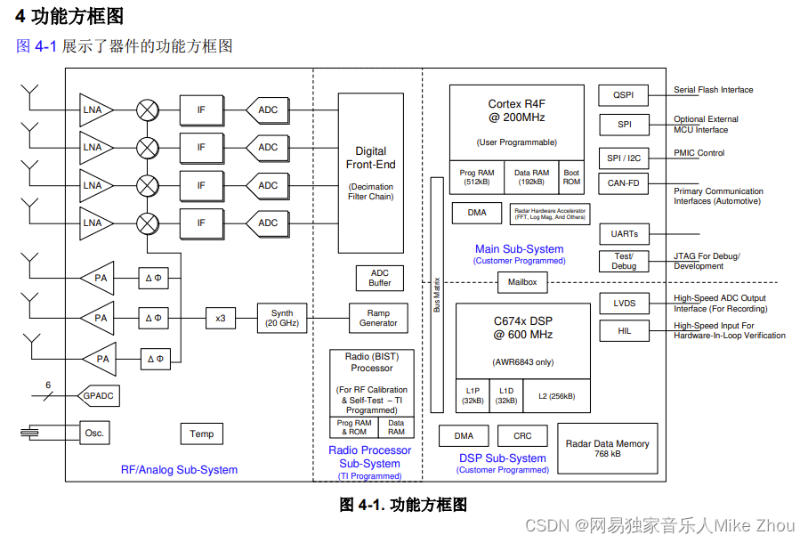
其中 大部分外设可以被MSS或DSS调用
另外 雷达前端BSS部分在SDK里由MMWave API调用

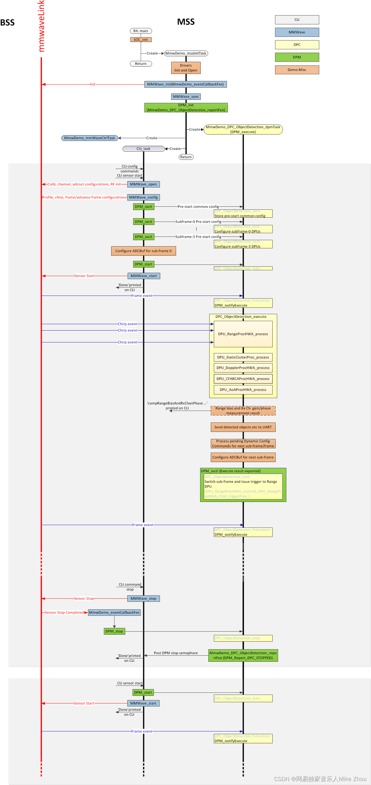
代码框架上 可以分成两个代码 MSS和DSS 两个代码同时运行 通过某些外设进行同步 协同运作

但也可以只跑一个内核 在仅MSS模式下 依旧可以调用某些用于信号处理的外设 demo代码就是如此

如下图为demo代码流程

Demo工程功能

IWR6843AOP的开箱工程是根据IWR6843AOPEVM开发板来的
该工程可以将IWR6843AOP的两个串口利用起来 实现的功能主要是两个方面：
通过115200波特率的串口配置参数 建立握手协议
通过115200*8的串口输出雷达数据
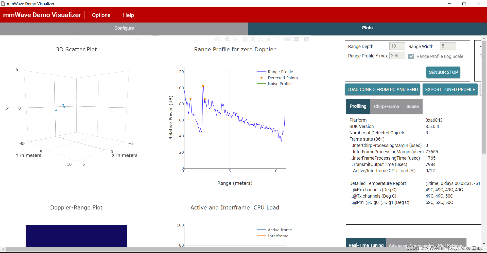
此工程需要匹配TI官方的上位机：mmWave_Demo_Visualizer_3.6.0来使用
该上位机可以在连接串口后自动化操作 并且对雷达数据可视化



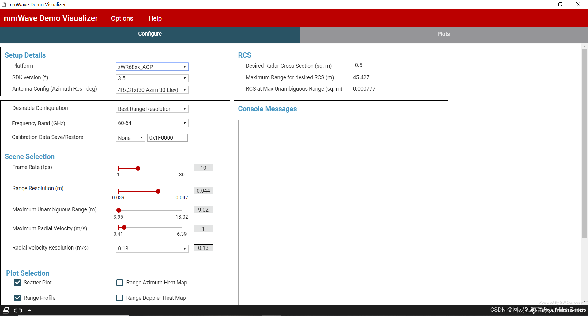
关于雷达参数配置 则在SDK的mmw\profiles目录下
言简意赅 可以直接更改该目录下的文件参数来达到配置雷达参数的目的

但这种方法不利于直接更改 每次用上位机运行后的参数是固定的（上位机运行需要SDK环境） 所以也可以在代码中写死 本文探讨的就是这个方向

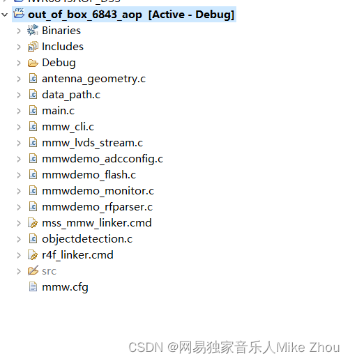
CCS工程导入

首先 在工业雷达包目录下找到该工程设置

C:\ti\mmwave_industrial_toolbox_4_12_0\labs\Out_Of_Box_Demo\src\xwr6843AOP

使用CCS的import project功能导入工程后 即可完成环境搭建

这里用到的SDK最新版为3.6版本

工程叙述

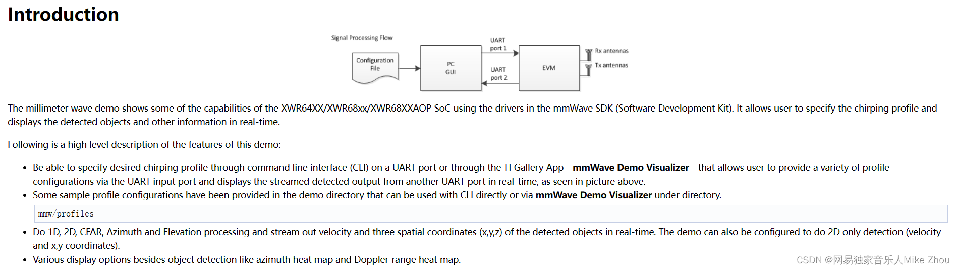
以下来自官方文档 可以直接跳过

Software Tasks

The demo consists of the following (SYSBIOS) tasks:

MmwDemo_initTask. This task is created/launched by main and is a one-time active task whose main functionality is to initialize drivers (<driver>_init), MMWave module (MMWave_init), DPM module (DPM_init), open UART and data path related drivers (EDMA, HWA), and create/launch the following tasks (the CLI_task is launched indirectly by calling CLI_open).
CLI_task. This command line interface task provides a simplified 'shell' interface which allows the configuration of the BSS via the mmWave interface (MMWave_config). It parses input CLI configuration commands like chirp profile and GUI configuration. When sensor start CLI command is parsed, all actions related to starting sensor and starting the processing the data path are taken. When sensor stop CLI command is parsed, all actions related to stopping the sensor and stopping the processing of the data path are taken
MmwDemo_mmWaveCtrlTask. This task is used to provide an execution context for the mmWave control, it calls in an endless loop the MMWave_execute API.
MmwDemo_DPC_ObjectDetection_dpmTask. This task is used to provide an execution context for DPM (Data Path Manager) execution, it calls in an endless loop the DPM_execute API. In this context, all of the registered object detection DPC (Data Path Chain) APIs like configuration, control and execute will take place. In this task. When the DPC's execute API produces the detected objects and other results, they are transmitted out of the UART port for display using the visualizer.

Data Path

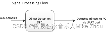
Top Level Data Path Processing Chain

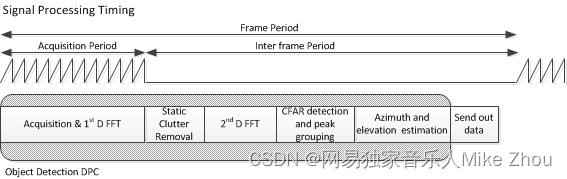
Top Level Data Path Timing

The data path processing consists of taking ADC samples as input and producing detected objects (point-cloud and other information) to be shipped out of UART port to the PC. The algorithm processing is realized using the DPM registered Object Detection DPC. The details of the processing in DPC can be seen from the following doxygen documentation:

ti/datapath/dpc/objectdetection/objdethwa/docs/doxygen/html/index.html

Output information sent to host

Output packets with the detection information are sent out every frame through the UART. Each packet consists of the header MmwDemo_output_message_header_t and the number of TLV items containing various data information with types enumerated in MmwDemo_output_message_type_e. The numerical values of the types can be found in mmw_output.h. Each TLV item consists of type, length (MmwDemo_output_message_tl_t) and payload information. The structure of the output packet is illustrated in the following figure. Since the length of the packet depends on the number of detected objects it can vary from frame to frame. The end of the packet is padded so that the total packet length is always multiple of 32 Bytes.

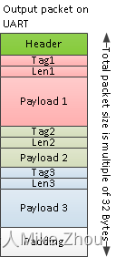
Output packet structure sent to UART
The following subsections describe the structure of each TLV.

List of detected objects

Type: (MMWDEMO_OUTPUT_MSG_DETECTED_POINTS)Length: (Number of detected objects) x (size of DPIF_PointCloudCartesian_t)Value: Array of detected objects. The information of each detected object is as per the structure DPIF_PointCloudCartesian_t. When the number of detected objects is zero, this TLV item is not sent. The maximum number of objects that can be detected in a sub-frame/frame is DPC_OBJDET_MAX_NUM_OBJECTS.The orientation of x,y and z axes relative to the sensor is as per the following figure. (Note: The antenna arrangement in the figure is shown for standard EVM (see gAntDef_default) as an example but the figure is applicable for any antenna arrangement.)

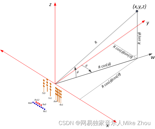
Coordinate Geometry
The whole detected objects TLV structure is illustrated in figure below.

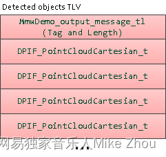
Detected objects TLV

Range profile

Type: (MMWDEMO_OUTPUT_MSG_RANGE_PROFILE)Length: (Range FFT size) x (size of uint16_t)Value: Array of profile points at 0th Doppler (stationary objects). The points represent the sum of log2 magnitudes of received antennas expressed in Q9 format.Noise floor profile
Type: (MMWDEMO_OUTPUT_MSG_NOISE_PROFILE)Length: (Range FFT size) x (size of uint16_t)Value: This is the same format as range profile but the profile is at the maximum Doppler bin (maximum speed objects). In general for stationary scene, there would be no objects or clutter at maximum speed so the range profile at such speed represents the receiver noise floor.

Azimuth static heatmap

Type: (MMWDEMO_OUTPUT_MSG_AZIMUT_STATIC_HEAT_MAP)Length: (Range FFT size) x (Number of "azimuth" virtual antennas) (size of cmplx16ImRe_t_)Value: Array DPU_AoAProcHWA_HW_Resources::azimuthStaticHeatMap. The antenna data are complex symbols, with imaginary first and real second in the following order:

Imag(ant 0, range 0), Real(ant 0, range 0),...,Imag(ant N-1, range 0),Real(ant N-1, range 0)...Imag(ant 0, range R-1), Real(ant 0, range R-1),...,Imag(ant N-1, range R-1),Real(ant N-1, range R-1)

Note that the number of virtual antennas is equal to the number of “azimuth” virtual antennas. The antenna symbols are arranged in the order as they occur at the input to azimuth FFT. Based on this data the static azimuth heat map could be constructed by the GUI running on the host.

Azimuth/Elevation static heatmap

Type: (MMWDEMO_OUTPUT_MSG_AZIMUT_ELEVATION_STATIC_HEAT_MAP)Length: (Range FFT size) x (Number of all virtual antennas) (size of cmplx16ImRe_t_)Value: Array DPU_AoAProcHWA_HW_Resources::azimuthStaticHeatMap. The antenna data are complex symbols, with imaginary first and real second in the following order:

 Imag(ant 0, range 0), Real(ant 0, range 0),...,Imag(ant N-1, range 0),Real(ant N-1, range 0)...Imag(ant 0, range R-1), Real(ant 0, range R-1),...,Imag(ant N-1, range R-1),Real(ant N-1, range R-1)

Note that the number of virtual antennas is equal to the total number of active virtual antennas. The antenna symbols are arranged in the order as they occur in the radar cube matrix. This TLV is sent by AOP version of MMW demo, that uses AOA2D DPU. Based on this data the static azimuth or elevation heat map could be constructed by the GUI running on the host.

Range/Doppler heatmap

Type: (MMWDEMO_OUTPUT_MSG_RANGE_DOPPLER_HEAT_MAP)Length: (Range FFT size) x (Doppler FFT size) (size of uint16_t)Value: Detection matrix DPIF_DetMatrix::data. The order is :

 X(range bin 0, Doppler bin 0),...,X(range bin 0, Doppler bin D-1),...X(range bin R-1, Doppler bin 0),...,X(range bin R-1, Doppler bin D-1)

Stats information

Type: (MMWDEMO_OUTPUT_MSG_STATS )Length: (size of MmwDemo_output_message_stats_t)Value: Timing information as per MmwDemo_output_message_stats_t. See timing diagram below related to the stats.

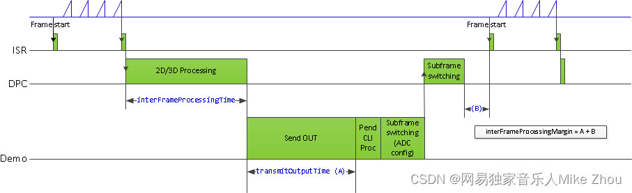
Processing timing

Note:The MmwDemo_output_message_stats_t::interChirpProcessingMargin is not computed (it is always set to 0). This is because there is no CPU involvement in the 1D processing (only HWA and EDMA are involved), and it is not possible to know how much margin is there in chirp processing without CPU being notified at every chirp when processing begins (chirp event) and when the HWA-EDMA computation ends. The CPU is intentionally kept free during 1D processing because a real application may use this time for doing some post-processing algorithm execution.
While the MmwDemo_output_message_stats_t::interFrameProcessingTime reported will be of the current sub-frame/frame, the MmwDemo_output_message_stats_t::interFrameProcessingMargin and MmwDemo_output_message_stats_t::transmitOutputTime will be of the previous sub-frame (of the same MmwDemo_output_message_header_t::subFrameNumber as that of the current sub-frame) or of the previous frame.
The MmwDemo_output_message_stats_t::interFrameProcessingMargin excludes the UART transmission time (available as MmwDemo_output_message_stats_t::transmitOutputTime). This is done intentionally to inform the user of a genuine inter-frame processing margin without being influenced by a slow transport like UART, this transport time can be significantly longer for example when streaming out debug information like heat maps. Also, in a real product deployment, higher speed interfaces (e.g LVDS) are likely to be used instead of UART. User can calculate the margin that includes transport overhead (say to determine the max frame rate that a particular demo configuration will allow) using the stats because they also contain the UART transmission time.

The CLI command “guMonitor” specifies which TLV element will be sent out within the output packet. The arguments of the CLI command are stored in the structure MmwDemo_GuiMonSel_t.

Side information of detected objects

Type: (MMWDEMO_OUTPUT_MSG_DETECTED_POINTS_SIDE_INFO)Length: (Number of detected objects) x (size of DPIF_PointCloudSideInfo_t)Value: Array of detected objects side information. The side information of each detected object is as per the structure DPIF_PointCloudSideInfo_t). When the number of detected objects is zero, this TLV item is not sent.

Temperature Stats

Type: (MMWDEMO_OUTPUT_MSG_TEMPERATURE_STATS)Length: (size of MmwDemo_temperatureStats_t)Value: Structure of detailed temperature report as obtained from Radar front end. MmwDemo_temperatureStats_t::tempReportValid is set to return value of rlRfGetTemperatureReport. If MmwDemo_temperatureStats_t::tempReportValid is 0, values in MmwDemo_temperatureStats_t::temperatureReport are valid else they should be ignored. This TLV is sent along with Stats TLV described in Stats information

Range Bias and Rx Channel Gain/Phase Measurement and Compensation

Because of imperfections in antenna layouts on the board, RF delays in SOC, etc, there is need to calibrate the sensor to compensate for bias in the range estimation and receive channel gain and phase imperfections. The following figure illustrates the calibration procedure.

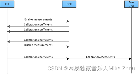
Calibration procedure ladder diagram

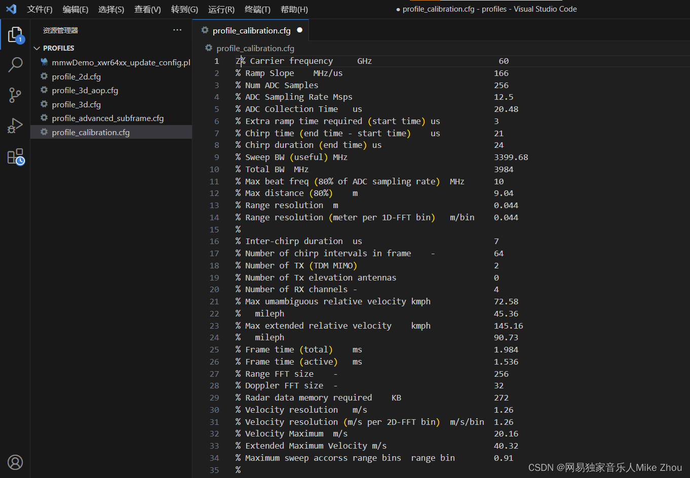
The calibration procedure includes the following steps:Set a strong target like corner reflector at the distance of X meter (X less than 50 cm is not recommended) at boresight.
Set the following command in the configuration profile in .../profiles/profile_calibration.cfg, to reflect the position X as follows: where D (in meters) is the distance of window around X where the peak will be searched. The purpose of the search window is to allow the test environment from not being overly constrained say because it may not be possible to clear it of all reflectors that may be stronger than the one used for calibration. The window size is recommended to be at least the distance equivalent of a few range bins. One range bin for the calibration profile (profile_calibration.cfg) is about 5 cm. The first argument "1" is to enable the measurement. The stated configuration profile (.cfg) must be used otherwise the calibration may not work as expected (this profile ensures all transmit and receive antennas are engaged among other things needed for calibration).measureRangeBiasAndRxChanPhase 1 X D
Start the sensor with the configuration file.
In the configuration file, the measurement is enabled because of which the DPC will be configured to perform the measurement and generate the measurement result (DPU_AoAProc_compRxChannelBiasCfg_t) in its result structure (DPC_ObjectDetection_ExecuteResult_t::compRxChanBiasMeasurement), the measurement results are written out on the CLI port (MmwDemo_measurementResultOutput) in the format below: For details of how DPC performs the measurement, see the DPC documentation.compRangeBiasAndRxChanPhase <rangeBias> <Re(0,0)> <Im(0,0)> <Re(0,1)> <Im(0,1)> ... <Re(0,R-1)> <Im(0,R-1)> <Re(1,0)> <Im(1,0)> ... <Re(T-1,R-1)> <Im(T-1,R-1)>
The command printed out on the CLI now can be copied and pasted in any configuration file for correction purposes. This configuration will be passed to the DPC for the purpose of applying compensation during angle computation, the details of this can be seen in the DPC documentation. If compensation is not desired, the following command should be given (depending on the EVM and antenna arrangement) Above sets the range bias to 0 and the phase coefficients to unity so that there is no correction. Note the two commands must always be given in any configuration file, typically the measure commmand will be disabled when the correction command is the desired one.For ISK EVM:compRangeBiasAndRxChanPhase 0.0   1 0 1 0 1 0 1 0 1 0 1 0 1 0 1 0 1 0 1 0 1 0 1 0 For AOP EVMcompRangeBiasAndRxChanPhase 0.0   1 0 -1 0 1 0 -1 0 1 0 -1 0 1 0 -1 0 1 0 -1 0 1 0 -1 0 

Streaming data over LVDS

The LVDS streaming feature enables the streaming of HW data (a combination of ADC/CP/CQ data) and/or user specific SW data through LVDS interface. The streaming is done mostly by the CBUFF and EDMA peripherals with minimal CPU intervention. The streaming is configured through the MmwDemo_LvdsStreamCfg_t CLI command which allows control of HSI header, enable/disable of HW and SW data and data format choice for the HW data. The choices for data formats for HW data are:MMW_DEMO_LVDS_STREAM_CFG_DATAFMT_DISABLED
MMW_DEMO_LVDS_STREAM_CFG_DATAFMT_ADC
MMW_DEMO_LVDS_STREAM_CFG_DATAFMT_CP_ADC_CQ
In order to see the high-level data format details corresponding to the above data format configurations, refer to the corresponding slides in ti\drivers\cbuff\docs\CBUFF_Transfers.pptxWhen HW data LVDS streaming is enabled, the ADC/CP/CQ data is streamed per chirp on every chirp event. When SW data streaming is enabled, it is streamed during inter-frame period after the list of detected objects for that frame is computed. The SW data streamed every frame/sub-frame is composed of the following in time:HSI header (HSIHeader_t): refer to HSI module for details.
User data header: MmwDemo_LVDSUserDataHeader
User data payloads:
Point-cloud information as a list : DPIF_PointCloudCartesian_t x number of detected objects
Point-cloud side information as a list : DPIF_PointCloudSideInfo_t x number of detected objects

The format of the SW data streamed is shown in the following figure:

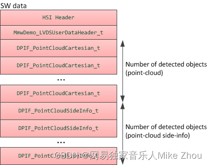
LVDS SW Data format

Note:Only single-chirp formats are allowed, multi-chirp is not supported.
When number of objects detected in frame/sub-frame is 0, there is no transmission beyond the user data header.
For HW data, the inter-chirp duration should be sufficient to stream out the desired amount of data. For example, if the HW data-format is ADC and HSI header is enabled, then the total amount of data generated per chirp is:
(numAdcSamples * numRxChannels * 4 (size of complex sample) + 52 [sizeof(HSIDataCardHeader_t) + sizeof(HSISDKHeader_t)] ) rounded up to multiples of 256 [=sizeof(HSIHeader_t)] bytes.
The chirp time Tc in us = idle time + ramp end time in the profile configuration. For n-lane LVDS with each lane at a maximum of B Mbps,
maximum number of bytes that can be send per chirp = Tc * n * B / 8 which should be greater than the total amount of data generated per chirp i.e
Tc * n * B / 8 >= round-up(numAdcSamples * numRxChannels * 4 + 52, 256).
E.g if n = 2, B = 600 Mbps, idle time = 7 us, ramp end time = 44 us, numAdcSamples = 512, numRxChannels = 4, then 7650 >= 8448 is violated so this configuration will not work. If the idle-time is doubled in the above example, then we have 8700 > 8448, so this configuration will work.
For SW data, the number of bytes to transmit each sub-frame/frame is:
52 [sizeof(HSIDataCardHeader_t) + sizeof(HSISDKHeader_t)] + sizeof(MmwDemo_LVDSUserDataHeader_t) [=8] +
number of detected objects (Nd) * { sizeof(DPIF_PointCloudCartesian_t) [=16] + sizeof(DPIF_PointCloudSideInfo_t) [=4] } rounded up to multiples of 256 [=sizeof(HSIHeader_t)] bytes.
or X = round-up(60 + Nd * 20, 256). So the time to transmit this data will be
X * 8 / (n*B) us. The maximum number of objects (Ndmax) that can be detected is defined in the DPC (DPC_OBJDET_MAX_NUM_OBJECTS). So if Ndmax = 500, then time to transmit SW data is 68 us. Because we parallelize this transmission with the much slower UART transmission, and because UART transmission is also sending at least the same amount of information as the LVDS, the LVDS transmission time will not add any burdens on the processing budget beyond the overhead of reconfiguring and activating the CBUFF session (this overhead is likely bigger than the time to transmit).
The total amount of data to be transmitted in a HW or SW packet must be greater than the minimum required by CBUFF, which is 64 bytes or 32 CBUFF Units (this is the definition CBUFF_MIN_TRANSFER_SIZE_CBUFF_UNITS in the CBUFF driver implementation). If this threshold condition is violated, the CBUFF driver will return an error during configuration and the demo will generate a fatal exception as a result. When HSI header is enabled, the total transfer size is ensured to be at least 256 bytes, which satisfies the minimum. If HSI header is disabled, for the HW session, this means that numAdcSamples * numRxChannels * 4 >= 64. Although mmwavelink allows minimum number of ADC samples to be 2, the demo is supported for numAdcSamples >= 64. So HSI header is not required to be enabled for HW only case. But if SW session is enabled, without the HSI header, the bytes in each packet will be 8 + Nd * 20. So for frames/sub-frames where Nd < 3, the demo will generate exception. Therefore HSI header must be enabled if SW is enabled, this is checked in the CLI command validation.

Implementation Notes

The LVDS implementation is mostly present in mmw_lvds_stream.h and mmw_lvds_stream.c with calls in mss_main.c. Additionally HSI clock initialization is done at first time sensor start using MmwDemo_mssSetHsiClk.
EDMA channel resources for CBUFF/LVDS are in the global resource file (mmw_res.h, see Hardware Resource Allocation) along with other EDMA resource allocation. The user data header and two user payloads are configured as three user buffers in the CBUFF driver. Hence SW allocation for EDMA provides for three sets of EDMA resources as seen in the SW part (swSessionEDMAChannelTable[.]) of MmwDemo_LVDSStream_EDMAInit. The maximum number of HW EDMA resources are needed for the data-format MMW_DEMO_LVDS_STREAM_CFG_DATAFMT_CP_ADC_CQ, which as seen in the corresponding slide in ti\drivers\cbuff\docs\CBUFF_Transfers.pptx is 12 channels (+ shadows) including the 1st special CBUFF EDMA event channel which CBUFF IP generates to the EDMA, hence the HW part (hwwSessionEDMAChannelTable[.]) of MmwDemo_LVDSStream_EDMAInit has 11 table entries.
Although the CBUFF driver is configured for two sessions (hw and sw), at any time only one can be active. So depending on the LVDS CLI configuration and whether advanced frame or not, there is logic to activate/deactivate HW and SW sessions as necessary.
The CBUFF session (HW/SW) configure-create and delete depends on whether or not re-configuration is required after the first time configuration.
For HW session, re-configuration is done during sub-frame switching to re-configure for the next sub-frame but when there is no advanced frame (number of sub-frames = 1), the HW configuration does not need to change so HW session does not need to be re-created.
For SW session, even though the user buffer start addresses and sizes of headers remains same, the number of detected objects which determines the sizes of some user buffers changes from one sub-frame/frame to another sub-frame/frame. Therefore SW session needs to be recreated every sub-frame/frame.
User may modify the application software to transmit different information than point-cloud in the SW data e.g radar cube data (output of range DPU). However the CBUFF also has a maximum link list entry size limit of 0x3FFF CBUFF units or 32766 bytes. This means it is the limit for each user buffer entry [there are maximum of 3 entries -1st used for user data header, 2nd for point-cloud and 3rd for point-cloud side information]. During session creation, if this limit is exceeded, the CBUFF will return an error (and demo will in turn generate an exception). A single physical buffer of say size 50000 bytes may be split across two user buffers by providing one user buffer with (address, size) = (start address, 25000) and 2nd user buffer with (address, size) = (start address + 25000, 25000), beyond this two (or three if user data header is also replaced) limit, the user will need to create and activate (and wait for completion) the SW session multiple times to accomplish the transmission.

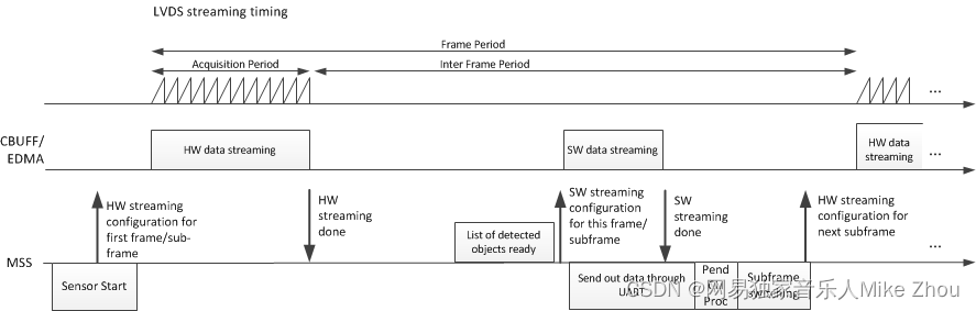
The following figure shows a timing diagram for the LVDS streaming (the figure is not to scale as actual durations will vary based on configuration).

How to bypass CLI

Re-implement the file mmw_cli.c as follows:MmwDemo_CLIInit should just create a task with input taskPriority. Lets say the task is called "MmwDemo_sensorConfig_task".
All other functions are not needed
Implement the MmwDemo_sensorConfig_task as follows:
Fill gMmwMCB.cfg.openCfg
Fill gMmwMCB.cfg.ctrlCfg
Add profiles and chirps using MMWave_addProfile and MMWave_addChirp functions
Call MmwDemo_CfgUpdate for every offset in Offsets for storing CLI configuration (MMWDEMO_xxx_OFFSET in mmw.h)
Fill gMmwMCB.dataPathObj.objDetCommonCfg.preStartCommonCfg
Call MmwDemo_openSensor
Call MmwDemo_startSensor (One can use helper function MmwDemo_isAllCfgInPendingState to know if all dynamic config was provided)

Hardware Resource Allocation

The Object Detection DPC needs to configure the DPUs hardware resources (HWA, EDMA). Even though the hardware resources currently are only required to be allocated for this one and only DPC in the system, the resource partitioning is shown to be in the ownership of the demo. This is to illustrate the general case of resource allocation across more than one DPCs and/or demo's own processing that is post-DPC processing. This partitioning can be seen in the mmw_res.h file. This file is passed as a compiler command line define

"--define=APP_RESOURCE_FILE="<ti/demo/xwr64xx/mmw/mmw_res.h>" 

in mmw.mak when building the DPC sources as part of building the demo application and is referred in object detection DPC sources where needed as

#include APP_RESOURCE_FILE