本文主要是介绍第R3周:天气预测,希望对大家解决编程问题提供一定的参考价值,需要的开发者们随着小编来一起学习吧!
- 🍨 本文为🔗365天深度学习训练营中的学习记录博客
🍖 原作者:K同学啊 | 接辅导、项目定制
- 🚀 文章来源:K同学的学习圈子
目录
我的环境
- 语言环境:python3.8.18
- 编译器:jupyter notebook
- 深度学习环境:Tensorflow
一、导入数据
import numpy as np
import pandas as pd
import seaborn as sns
import matplotlib.pyplot as plt
import warnings
warnings.filterwarnings('ignore')from sklearn.model_selection import train_test_split
from sklearn.preprocessing import MinMaxScaler
import tensorflow as tf
from tensorflow.keras.models import Sequential
from tensorflow.keras.layers import Dense, Activation,Dropout
from tensorflow.keras.callbacks import EarlyStopping
from sklearn.metrics import classification_report,confusion_matrix
from sklearn.metrics import r2_score
from sklearn.metrics import mean_absolute_error , mean_absolute_percentage_error , mean_squared_error
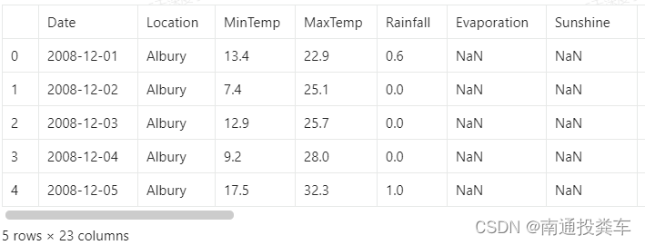
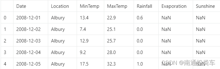
data = pd.read_csv("weatherAUS.csv")
df   = data.copy()
data.head()
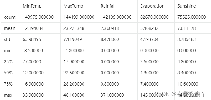
data.describe()
data.dtypes
Date              object
Location          object
MinTemp          float64
MaxTemp          float64
Rainfall         float64
Evaporation      float64
Sunshine         float64
WindGustDir       object
WindGustSpeed    float64
WindDir9am        object
WindDir3pm        object
WindSpeed9am     float64
WindSpeed3pm     float64
Humidity9am      float64
Humidity3pm      float64
Pressure9am      float64
Pressure3pm      float64
Cloud9am         float64
Cloud3pm         float64
Temp9am          float64
Temp3pm          float64
RainToday         object
RainTomorrow      object
dtype: object
data['Date'] = pd.to_datetime(data['Date'])
data['Date'].head() 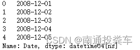
data['year']=data['Date'].dt.year
data['Month']=data['Date'].dt.month
data['day']=data['Date'].dt.day
data.head()
data.drop('Date',inplace=True,axis=1)
data.columns
Index(['Location', 'MinTemp', 'MaxTemp', 'Rainfall', 'Evaporation', 'Sunshine','WindGustDir', 'WindGustSpeed', 'WindDir9am', 'WindDir3pm','WindSpeed9am', 'WindSpeed3pm', 'Humidity9am', 'Humidity3pm','Pressure9am', 'Pressure3pm', 'Cloud9am', 'Cloud3pm', 'Temp9am','Temp3pm', 'RainToday', 'RainTomorrow', 'year', 'Month', 'day'],dtype='object')
二、探索式数据分析
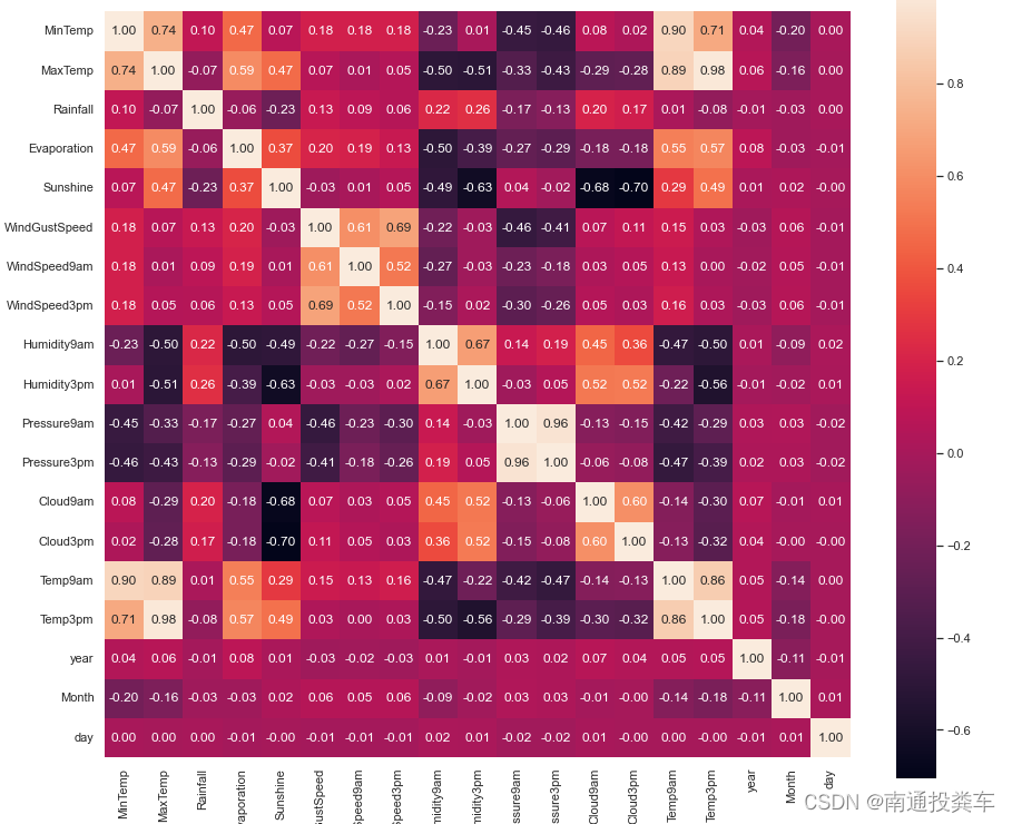
1.数据相关性探索
plt.figure(figsize=(15,13))
# data.corr()表示了data中的两个变量之间的相关性
ax = sns.heatmap(data.corr(), square=True, annot=True, fmt='.2f')
ax.set_xticklabels(ax.get_xticklabels(), rotation=90)
plt.show()
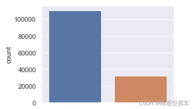
2.是否会下雨
sns.set(style="darkgrid")
plt.figure(figsize=(4,3))
sns.countplot(x='RainTomorrow',data=data)
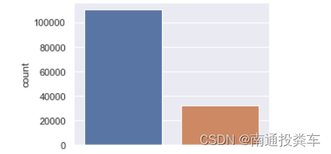
plt.figure(figsize=(4,3))
sns.countplot(x='RainToday',data=data)
x=pd.crosstab(data['RainTomorrow'],data['RainToday'])
x

y=x/x.transpose().sum().values.reshape(2,1)*100
y

如果今天不下雨,那么明天下雨的机会 = 15%
如果今天下雨明天下雨的机会 = 46%
y.plot(kind="bar",figsize=(4,3),color=['#006666','#d279a6']);

3.地理位置和下雨的关系
x=pd.crosstab(data['Location'],data['RainToday'])
# 获取每个城市下雨天数和非下雨天数的百分比
x
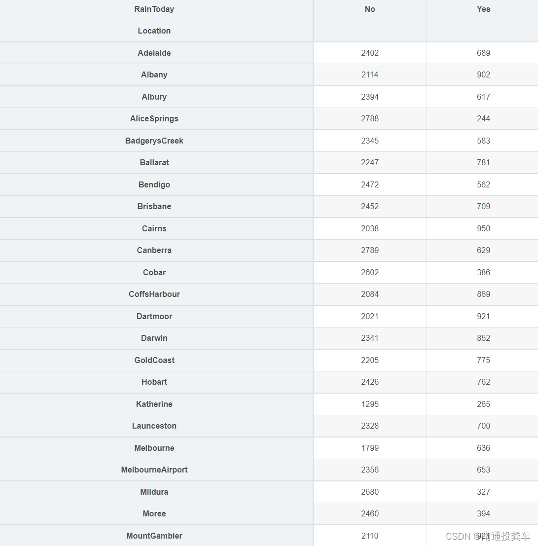
y=x/x.sum(axis=1).values.reshape((-1, 1))*100
# 按每个城市的雨天百分比排序
y=y.sort_values(by='Yes',ascending=True )color=['#cc6699','#006699','#006666','#862d86','#ff9966'  ]
y.Yes.plot(kind="barh",figsize=(15,20),color=color)

位置影响下雨,对于 Portland 来说,有 36% 的时间在下雨,而对于 Woomers 来说,只有6%的时间在下雨
4.湿度和压力对下雨的影响
data.columns
Index(['Location', 'MinTemp', 'MaxTemp', 'Rainfall', 'Evaporation', 'Sunshine','WindGustDir', 'WindGustSpeed', 'WindDir9am', 'WindDir3pm','WindSpeed9am', 'WindSpeed3pm', 'Humidity9am', 'Humidity3pm','Pressure9am', 'Pressure3pm', 'Cloud9am', 'Cloud3pm', 'Temp9am','Temp3pm', 'RainToday', 'RainTomorrow', 'year', 'Month', 'day'],dtype='object')
plt.figure(figsize=(8,6))
sns.scatterplot(data=data,x='Pressure9am',y='Pressure3pm',hue='RainTomorrow');
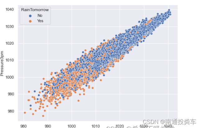
plt.figure(figsize=(8,6))
sns.scatterplot(data=data,x='Humidity9am',y='Humidity3pm',hue='RainTomorrow');
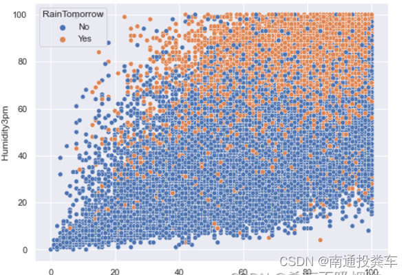
低压与高湿度会增加第二天下雨的概率,尤其是下午 3 点的空气湿度。
5.气温对下雨的影响
plt.figure(figsize=(8,6))
sns.scatterplot(x='MaxTemp', y='MinTemp', data=data, hue='RainTomorrow');

结论:当一天的最高气温和最低气温接近时,第二天下雨的概率会增加。
三.数据预处理
1.处理缺损值
# 每列中缺失数据的百分比
data.isnull().sum()/data.shape[0]*100
Location          0.000000
MinTemp           1.020899
MaxTemp           0.866905
Rainfall          2.241853
Evaporation      43.166506
Sunshine         48.009762
WindGustDir       7.098859
WindGustSpeed     7.055548
WindDir9am        7.263853
WindDir3pm        2.906641
WindSpeed9am      1.214767
WindSpeed3pm      2.105046
Humidity9am       1.824557
Humidity3pm       3.098446
Pressure9am      10.356799
Pressure3pm      10.331363
Cloud9am         38.421559
Cloud3pm         40.807095
Temp9am           1.214767
Temp3pm           2.481094
RainToday         2.241853
RainTomorrow      2.245978
year              0.000000
Month             0.000000
day               0.000000
dtype: float64
# 在该列中随机选择数进行填充
lst=['Evaporation','Sunshine','Cloud9am','Cloud3pm']
for col in lst:fill_list = data[col].dropna()data[col] = data[col].fillna(pd.Series(np.random.choice(fill_list, size=len(data.index))))
s = (data.dtypes == "object")
object_cols = list(s[s].index)
object_cols
['Location','WindGustDir','WindDir9am','WindDir3pm','RainToday','RainTomorrow']
# inplace=True:直接修改原对象,不创建副本
# data[i].mode()[0] 返回频率出现最高的选项,众数for i in object_cols:data[i].fillna(data[i].mode()[0], inplace=True)
t = (data.dtypes == "float64")
num_cols = list(t[t].index)
num_cols
['MinTemp','MaxTemp','Rainfall','Evaporation','Sunshine','WindGustSpeed','WindSpeed9am','WindSpeed3pm','Humidity9am','Humidity3pm','Pressure9am','Pressure3pm','Cloud9am','Cloud3pm','Temp9am','Temp3pm']
# .median(), 中位数
for i in num_cols:data[i].fillna(data[i].median(), inplace=True)
data.isnull().sum()
Location         0
MinTemp          0
MaxTemp          0
Rainfall         0
Evaporation      0
Sunshine         0
WindGustDir      0
WindGustSpeed    0
WindDir9am       0
WindDir3pm       0
WindSpeed9am     0
WindSpeed3pm     0
Humidity9am      0
Humidity3pm      0
Pressure9am      0
Pressure3pm      0
Cloud9am         0
Cloud3pm         0
Temp9am          0
Temp3pm          0
RainToday        0
RainTomorrow     0
year             0
Month            0
day              0
dtype: int64
2.构建数据集
from sklearn.preprocessing import LabelEncoderlabel_encoder = LabelEncoder()
for i in object_cols:data[i] = label_encoder.fit_transform(data[i])
X = data.drop(['RainTomorrow','day'],axis=1).values
y = data['RainTomorrow'].values
X_train, X_test, y_train, y_test = train_test_split(X,y,test_size=0.25,random_state=101)
scaler = MinMaxScaler()
scaler.fit(X_train)
X_train = scaler.transform(X_train)
X_test  = scaler.transform(X_test)
四.预测是否下雨
1.搭建神经网路
from tensorflow.keras.optimizers import Adammodel = Sequential()
model.add(Dense(units=24,activation='tanh',))
model.add(Dense(units=18,activation='tanh'))
model.add(Dense(units=23,activation='tanh'))
model.add(Dropout(0.5))
model.add(Dense(units=12,activation='tanh'))
model.add(Dropout(0.2))
model.add(Dense(units=1,activation='sigmoid'))optimizer = tf.keras.optimizers.Adam(learning_rate=1e-4)model.compile(loss='binary_crossentropy',optimizer=optimizer,metrics="accuracy")
early_stop = EarlyStopping(monitor='val_loss', mode='min',min_delta=0.001, verbose=1, patience=25,restore_best_weights=True)
2.模型训练
model.fit(x=X_train, y=y_train, validation_data=(X_test, y_test), verbose=1,callbacks=[early_stop],epochs = 10,batch_size = 32
)
Epoch 1/10
3410/3410 [==============================] - 8s 2ms/step - loss: 0.4570 - accuracy: 0.7996 - val_loss: 0.3916 - val_accuracy: 0.8283
Epoch 2/10
3410/3410 [==============================] - 8s 2ms/step - loss: 0.3962 - accuracy: 0.8304 - val_loss: 0.3774 - val_accuracy: 0.8356
Epoch 3/10
3410/3410 [==============================] - 8s 2ms/step - loss: 0.3887 - accuracy: 0.8351 - val_loss: 0.3776 - val_accuracy: 0.8379
Epoch 4/10
3410/3410 [==============================] - 8s 2ms/step - loss: 0.3840 - accuracy: 0.8372 - val_loss: 0.3724 - val_accuracy: 0.8389
Epoch 5/10
3410/3410 [==============================] - 8s 2ms/step - loss: 0.3814 - accuracy: 0.8382 - val_loss: 0.3734 - val_accuracy: 0.8394
Epoch 6/10
3410/3410 [==============================] - 8s 2ms/step - loss: 0.3794 - accuracy: 0.8391 - val_loss: 0.3697 - val_accuracy: 0.8399
Epoch 7/10
3410/3410 [==============================] - 8s 2ms/step - loss: 0.3791 - accuracy: 0.8393 - val_loss: 0.3692 - val_accuracy: 0.8408
Epoch 8/10
3410/3410 [==============================] - 8s 2ms/step - loss: 0.3774 - accuracy: 0.8395 - val_loss: 0.3686 - val_accuracy: 0.8411
Epoch 9/10
3410/3410 [==============================] - 8s 2ms/step - loss: 0.3771 - accuracy: 0.8398 - val_loss: 0.3680 - val_accuracy: 0.8410
Epoch 10/10
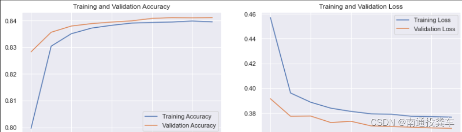
3410/3410 [==============================] - 8s 2ms/step - loss: 0.3767 - accuracy: 0.8395 - val_loss: 0.3677 - val_accuracy: 0.84113.结果可视化
import matplotlib.pyplot as pltacc = model.history.history['accuracy']
val_acc = model.history.history['val_accuracy']loss = model.history.history['loss']
val_loss = model.history.history['val_loss']epochs_range = range(10)plt.figure(figsize=(14, 4))
plt.subplot(1, 2, 1)plt.plot(epochs_range, acc, label='Training Accuracy')
plt.plot(epochs_range, val_acc, label='Validation Accuracy')
plt.legend(loc='lower right')
plt.title('Training and Validation Accuracy')plt.subplot(1, 2, 2)
plt.plot(epochs_range, loss, label='Training Loss')
plt.plot(epochs_range, val_loss, label='Validation Loss')
plt.legend(loc='upper right')
plt.title('Training and Validation Loss')
plt.show()
这篇关于第R3周:天气预测的文章就介绍到这儿,希望我们推荐的文章对编程师们有所帮助!