好好学习第三天：RNN与股票预测

本文主要是介绍好好学习第三天：RNN与股票预测，希望对大家解决编程问题提供一定的参考价值，需要的开发者们随着小编来一起学习吧！

>- 本文为[🔗365天深度学习训练营](https://mp.weixin.qq.com/s/k-vYaC8l7uxX51WoypLkTw) 中的学习记录博客
>- 参考文章地址： [🔗深度学习100例-循环神经网络（RNN）实现股票预测 | 第9天](https://mtyjkh.blog.csdn.net/article/details/117752046)

活动地址：CSDN21天学习挑战赛

一、RNN

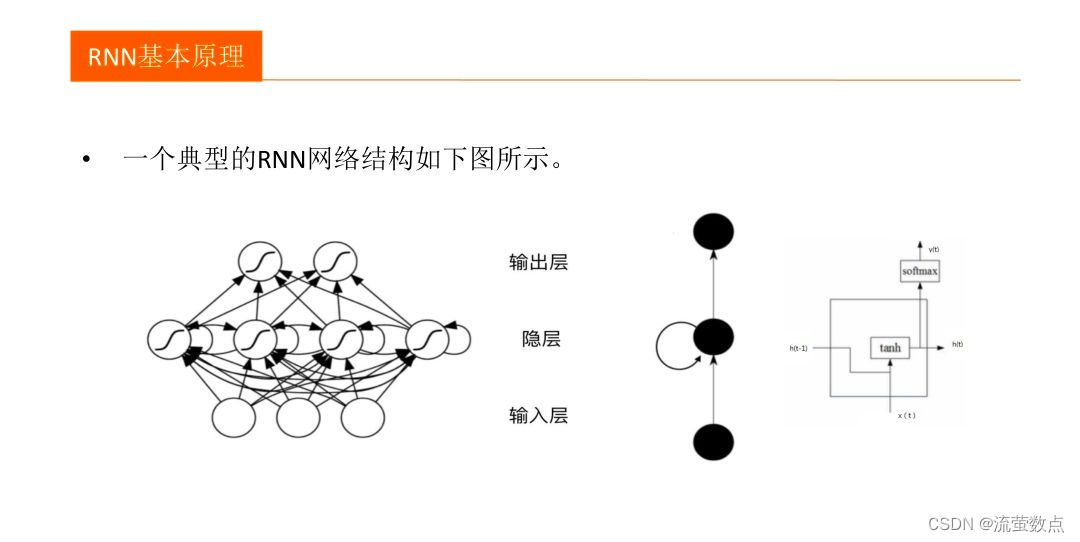
RNN（Recurrent Neural Network）循环神经网络是一种对序列数据建模的神经网络。RNN不同于前向神经网络，它的层内、层与层之间的信息可以双向传递，更高效地存储信息，利用更复杂的方法来更新规则，通常用于处理信息序列的任务。

RNN在自然语言处理、图像识别、语音识别、上下文的预测、在线交易预测、实时翻译等领域得到了大量的应用。

RNN主要用来处理序列数据，在传统的神经网络模型中，是从输入层到隐含层再到输出层，每层内的节点之间无连接，循环神经网络中一个当前神经元的输出与前面的输出也有关，网络会对前面的信息进行记忆并应用于当前神经元的计算中，隐藏层之间的节点是有连接的，并且隐藏层的输入不仅包含输入层的输出还包含上一时刻隐藏层的输出。理论上，RNN可以对任意长度的序列数据进行处理。

RNN缺陷：长期依赖问题，产生长跨度依赖问题。

RNN分类：

（1）输入一个输出多个，例如输入一张图像，输出这张图像的描述信息。

（2）输入是多个，输出则是一个，例如输入段话，输出这段话的情感。

（3）输入是多个，输出也是多个，如机器翻译输入一段话输出也是一段话（多个词）。

（4）多个输入和输出是同步的，例如进行字幕标记。

二、过程

1.导入库

import os,math
from tensorflow.keras.layers import Dropout, Dense, SimpleRNN
from sklearn.preprocessing   import MinMaxScaler
from sklearn                 import metrics
import numpy             as np
import pandas            as pd
import tensorflow        as tf
import matplotlib.pyplot as plt
# 支持中文
plt.rcParams['font.sans-serif'] = ['SimHei']  # 用来正常显示中文标签
plt.rcParams['axes.unicode_minus'] = False  # 用来正常显示负号

2.导入数据

data = pd.read_csv('SH600519.csv')  # 读取股票文件data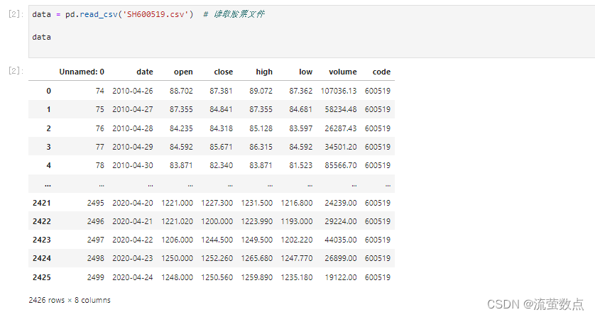

3.划分训练集和测试集

iloc[行索引位置,列索引位置]

"""
前(2426-300=2126)天的开盘价作为训练集,表格从0开始计数，2:3 是提取[2:3)列，前闭后开,故提取出C列开盘价
后300天的开盘价作为测试集
"""
training_set = data.iloc[0:2426 - 300, 2:3].values  
test_set = data.iloc[2426 - 300:, 2:3].values

4.归一化

MinMaxScaler()函数在preprocessing模块，用来实现数据的归一化，即把数据映射到 [ 0，1 ] 。

sc           = MinMaxScaler(feature_range=(0, 1))
training_set = sc.fit_transform(training_set)
test_set     = sc.transform(test_set)

5.设置测试集训练集

x_train = []
y_train = []x_test = []
y_test = []"""
使用前60天的开盘价作为输入特征x_train第61天的开盘价作为输入标签y_trainfor循环共构建2426-300-60=2066组训练数据。共构建300-60=260组测试数据
"""
for i in range(60, len(training_set)):x_train.append(training_set[i - 60:i, 0])y_train.append(training_set[i, 0])for i in range(60, len(test_set)):x_test.append(test_set[i - 60:i, 0])y_test.append(test_set[i, 0])# 对训练集进行打乱
np.random.seed(7)
np.random.shuffle(x_train)
np.random.seed(7)
np.random.shuffle(y_train)
tf.random.set_random_seed(7)  #此句修改

6.调整数据

"""
将训练数据调整为数组（array）调整后的形状：
x_train:(2066, 60, 1)
y_train:(2066,)
x_test :(240, 60, 1)
y_test :(240,)
"""
x_train, y_train = np.array(x_train), np.array(y_train) # x_train形状为：(2066, 60, 1)
x_test,  y_test  = np.array(x_test),  np.array(y_test)"""
输入要求：[送入样本数， 循环核时间展开步数， 每个时间步输入特征个数]
"""
x_train = np.reshape(x_train, (x_train.shape[0], 60, 1))
x_test  = np.reshape(x_test,  (x_test.shape[0], 60, 1))

7.构建模型

model = tf.keras.Sequential([SimpleRNN(100, return_sequences=True), #布尔值。是返回输出序列中的最后一个输出，还是全部序列。Dropout(0.1),                         #防止过拟合SimpleRNN(100),Dropout(0.1),Dense(1)
])

8.激活模型

# 该应用只观测loss数值，不观测准确率，所以删去metrics选项，一会在每个epoch迭代显示时只显示loss值
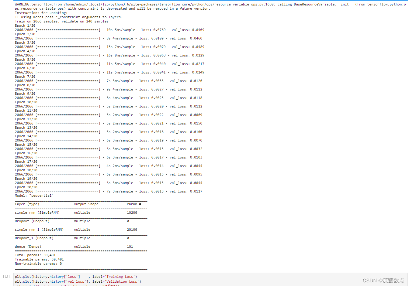
model.compile(optimizer=tf.keras.optimizers.Adam(0.001),loss='mean_squared_error')  # 损失函数用均方误差

9.模型训练

history = model.fit(x_train, y_train, batch_size=64, epochs=20, validation_data=(x_test, y_test), validation_freq=1)                  #测试的epoch间隔数model.summary()

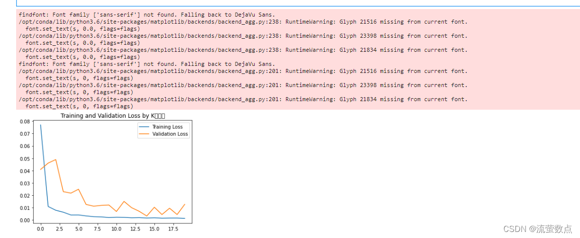
10.可视化——绘制loss图

plt.plot(history.history['loss']    , label='Training Loss')
plt.plot(history.history['val_loss'], label='Validation Loss')
plt.title('Training and Validation Loss by K同学啊')
plt.legend()
plt.show()

11.预测

X=scaler.inverse_transform(X)

将标准化后的数据转换为原始数据。

predicted_stock_price = model.predict(x_test)                       # 测试集输入模型进行预测
predicted_stock_price = sc.inverse_transform(predicted_stock_price) # 对预测数据还原---从（0，1）反归一化到原始范围
real_stock_price = sc.inverse_transform(test_set[60:])              # 对真实数据还原---从（0，1）反归一化到原始范围# 画出真实数据和预测数据的对比曲线
plt.plot(real_stock_price, color='red', label='Stock Price')
plt.plot(predicted_stock_price, color='blue', label='Predicted Stock Price')
plt.title('Stock Price Prediction by K同学啊')
plt.xlabel('Time')
plt.ylabel('Stock Price')
plt.legend()
plt.show()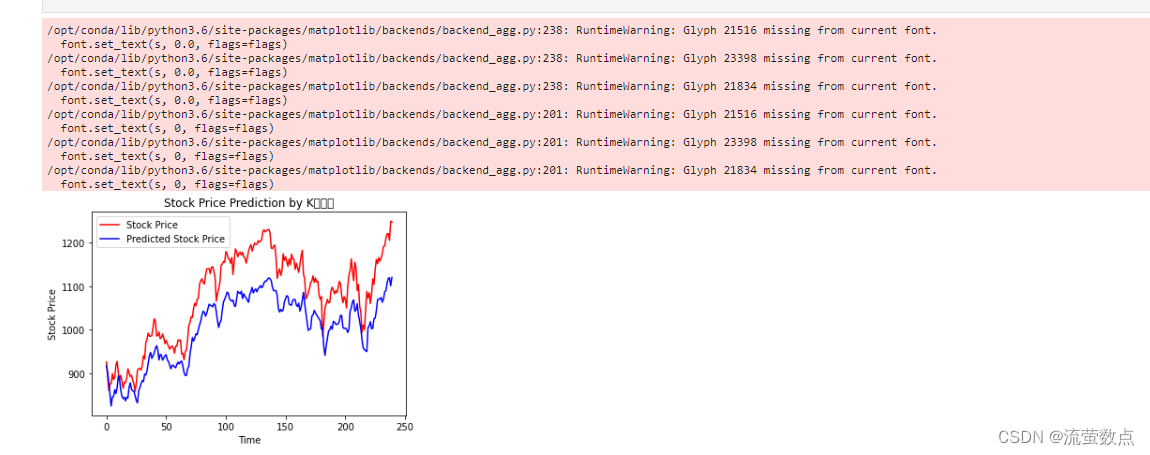

12.评估

"""
MSE  ：均方误差    ----->  预测值减真实值求平方后求均值
RMSE ：均方根误差  ----->  对均方误差开方
MAE  ：平均绝对误差----->  预测值减真实值求绝对值后求均值
R2   ：决定系数，可以简单理解为反映模型拟合优度的重要的统计量详细介绍可以参考文章：https://blog.csdn.net/qq_38251616/article/details/107997435
"""
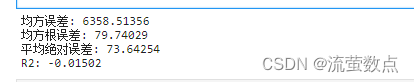
MSE   = metrics.mean_squared_error(predicted_stock_price, real_stock_price)
RMSE  = metrics.mean_squared_error(predicted_stock_price, real_stock_price)**0.5
MAE   = metrics.mean_absolute_error(predicted_stock_price, real_stock_price)
R2    = metrics.r2_score(predicted_stock_price, real_stock_price)print('均方误差: %.5f' % MSE)
print('均方根误差: %.5f' % RMSE)
print('平均绝对误差: %.5f' % MAE)
print('R2: %.5f' % R2)