本文主要是介绍葡萄酒数据集的随机森林分类,希望对大家解决编程问题提供一定的参考价值,需要的开发者们随着小编来一起学习吧!
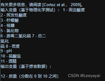
一:数据集介绍
1:数据集下载
https://archive.ics.uci.edu/ml/datasets/Wine+Quality

我这里选择的是红酒样本
数据的特征与标签
特征:11个 ; 标签:红酒质量0-10之间,11个类别
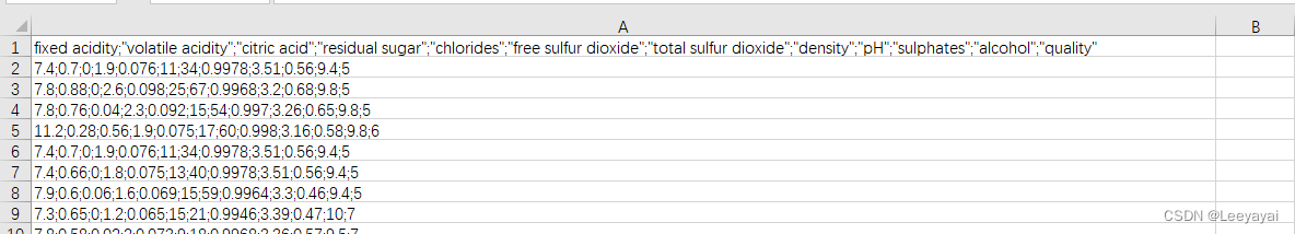
2:查看数据集
可以看到数据都在一列里,需要改一下
二:数据处理
1:数据分列
观察数据,在一列里用分号隔开,由此对数据分列
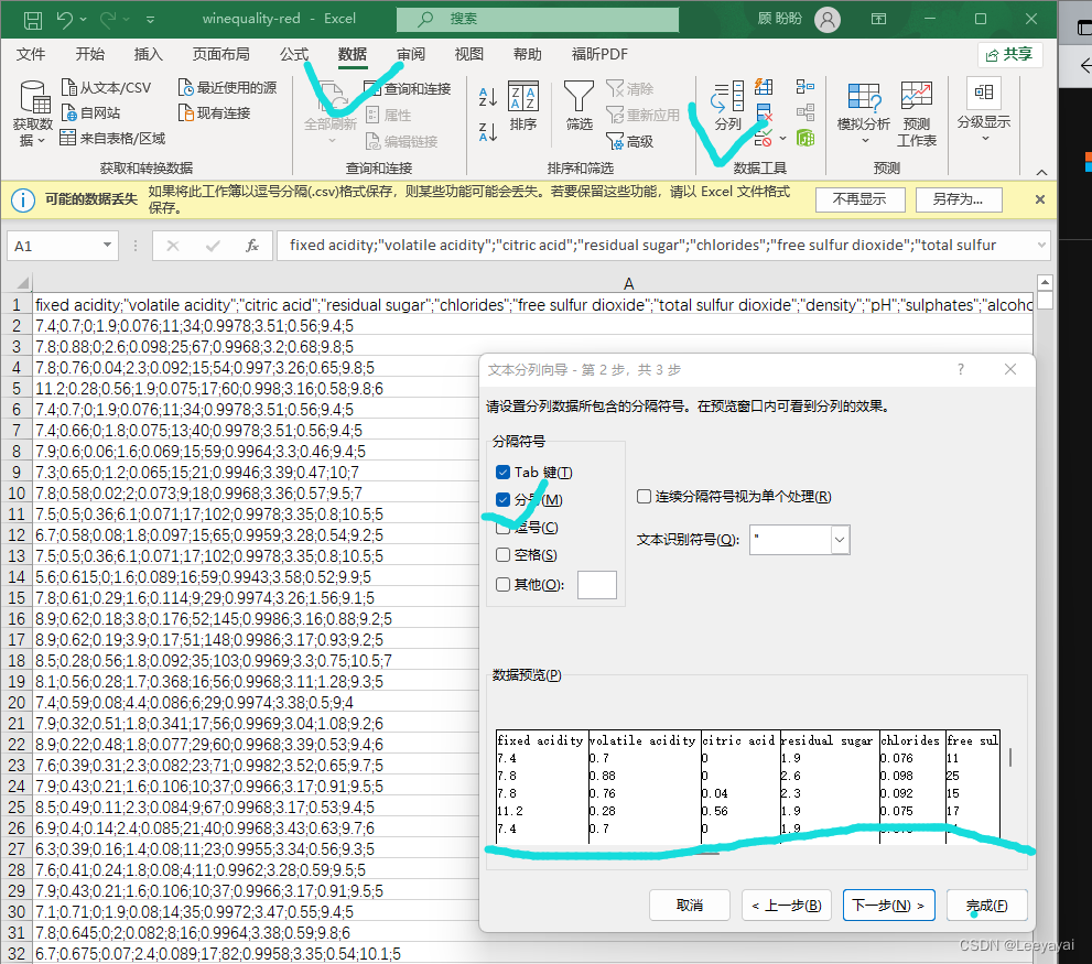
选定需要分列的数据–选数据菜单–分列–分隔符–选分号–OK
分列后的数据

2:导入数据
import pandas as pd
#获取数据
data = pd.read_csv("F:\\书籍学习:python数据挖掘与机器学习实战\\葡萄酒数据集的随机森林分类\\winequality-red.csv")
data.head()#查看数据
| fixed acidity | volatile acidity | citric acid | residual sugar | chlorides | free sulfur dioxide | total sulfur dioxide | density | pH | sulphates | alcohol | quality | |
|---|---|---|---|---|---|---|---|---|---|---|---|---|
| 0 | 7.4 | 0.70 | 0.00 | 1.9 | 0.076 | 11.0 | 34.0 | 0.9978 | 3.51 | 0.56 | 9.4 | 5 |
| 1 | 7.8 | 0.88 | 0.00 | 2.6 | 0.098 | 25.0 | 67.0 | 0.9968 | 3.20 | 0.68 | 9.8 | 5 |
| 2 | 7.8 | 0.76 | 0.04 | 2.3 | 0.092 | 15.0 | 54.0 | 0.9970 | 3.26 | 0.65 | 9.8 | 5 |
| 3 | 11.2 | 0.28 | 0.56 | 1.9 | 0.075 | 17.0 | 60.0 | 0.9980 | 3.16 | 0.58 | 9.8 | 6 |
| 4 | 7.4 | 0.70 | 0.00 | 1.9 | 0.076 | 11.0 | 34.0 | 0.9978 | 3.51 | 0.56 | 9.4 | 5 |
# 导入所有需要的库import numpy as np
import pandas as pd
from sklearn.ensemble import RandomForestClassifier
3:将数据拆分为特征与标签
features = data.drop('quality', 1)
# df = data.iloc[:, :11] #取前11列数据
labels = data['quality']
print(features.shape)
print(labels.shape)
(1599, 11)
(1599,)C:\Users\Hp\AppData\Local\Temp\ipykernel_12320\351942566.py:1: FutureWarning: In a future version of pandas all arguments of DataFrame.drop except for the argument 'labels' will be keyword-only.features = data.drop('quality', 1)
三:数据分析
1:数据的描述性分析
# 描述性分析
print(features.describe())# 直方图
# hist(),输出各个特征对比的直方图
features.hist()
       fixed acidity  volatile acidity  citric acid  residual sugar  \
count    1599.000000       1599.000000  1599.000000     1599.000000
mean        8.319637          0.527821     0.270976        2.538806
std         1.741096          0.179060     0.194801        1.409928
min         4.600000          0.120000     0.000000        0.900000
25%         7.100000          0.390000     0.090000        1.900000
50%         7.900000          0.520000     0.260000        2.200000
75%         9.200000          0.640000     0.420000        2.600000
max        15.900000          1.580000     1.000000       15.500000   chlorides  free sulfur dioxide  total sulfur dioxide      density  \
count  1599.000000          1599.000000           1599.000000  1599.000000
mean      0.087467            15.874922             46.467792     0.996747
std       0.047065            10.460157             32.895324     0.001887
min       0.012000             1.000000              6.000000     0.990070
25%       0.070000             7.000000             22.000000     0.995600
50%       0.079000            14.000000             38.000000     0.996750
75%       0.090000            21.000000             62.000000     0.997835
max       0.611000            72.000000            289.000000     1.003690   pH    sulphates      alcohol
count  1599.000000  1599.000000  1599.000000
mean      3.311113     0.658149    10.422983
std       0.154386     0.169507     1.065668
min       2.740000     0.330000     8.400000
25%       3.210000     0.550000     9.500000
50%       3.310000     0.620000    10.200000
75%       3.400000     0.730000    11.100000
max       4.010000     2.000000    14.900000  array([[<AxesSubplot:title={'center':'fixed acidity'}>,<AxesSubplot:title={'center':'volatile acidity'}>,<AxesSubplot:title={'center':'citric acid'}>],[<AxesSubplot:title={'center':'residual sugar'}>,<AxesSubplot:title={'center':'chlorides'}>,<AxesSubplot:title={'center':'free sulfur dioxide'}>],[<AxesSubplot:title={'center':'total sulfur dioxide'}>,<AxesSubplot:title={'center':'density'}>,<AxesSubplot:title={'center':'pH'}>],[<AxesSubplot:title={'center':'sulphates'}>,<AxesSubplot:title={'center':'alcohol'}>, <AxesSubplot:>]],dtype=object)

2:各等级酒的描述性分析
分为三个等级:低级(0-3),中级(4-7),高级(8-10)
(最大最小值,平均值,标准差)
2.1: 统计表类别个数df.value_counts()
#查看标签值,有几类标签print(labels.value_counts())
5    681
6    638
7    199
4     53
8     18
3     10
Name: quality, dtype: int64
2.2:对数据进行分割,低级,中级,高级红酒
暂放-
3 :变量的相关性分析
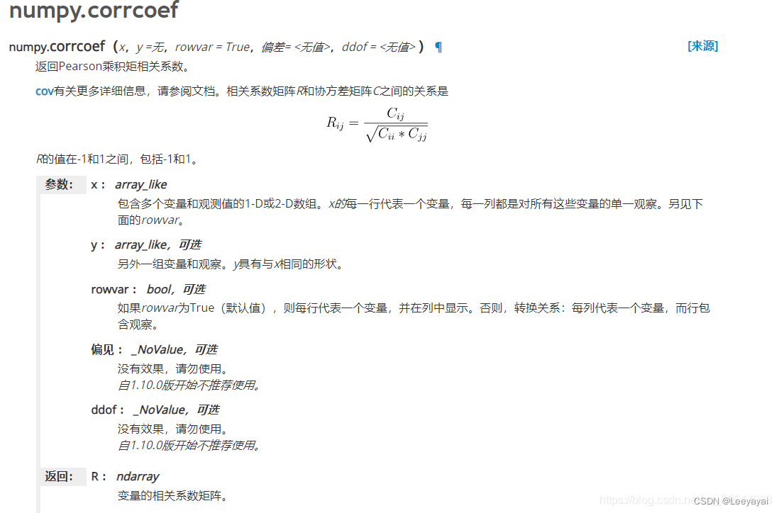
1:np.corrcoef()
#features = data.drop('quality', 1)
df = data.iloc[:, :11] #取前11列数据
#print(df.head())#查看前5列数据#分析两个变量间的相关性
print(np.corrcoef(data.iloc[1], data.iloc[2]))#分析所有变量之间的相关性
print(np.corrcoef(df, rowvar = False))
[[1.         0.99368451][0.99368451 1.        ]]
[[ 1.         -0.25613089  0.67170343  0.11477672  0.09370519 -0.15379419-0.11318144  0.66804729 -0.68297819  0.18300566 -0.06166827][-0.25613089  1.         -0.55249568  0.00191788  0.06129777 -0.010503830.07647     0.02202623  0.23493729 -0.26098669 -0.20228803][ 0.67170343 -0.55249568  1.          0.14357716  0.20382291 -0.060978130.03553302  0.36494718 -0.54190414  0.31277004  0.10990325][ 0.11477672  0.00191788  0.14357716  1.          0.05560954  0.1870490.20302788  0.35528337 -0.08565242  0.00552712  0.04207544][ 0.09370519  0.06129777  0.20382291  0.05560954  1.          0.005562150.04740047  0.20063233 -0.26502613  0.37126048 -0.22114054][-0.15379419 -0.01050383 -0.06097813  0.187049    0.00556215  1.0.66766645 -0.02194583  0.0703775   0.05165757 -0.06940835][-0.11318144  0.07647     0.03553302  0.20302788  0.04740047  0.667666451.          0.07126948 -0.06649456  0.04294684 -0.20565394][ 0.66804729  0.02202623  0.36494718  0.35528337  0.20063233 -0.021945830.07126948  1.         -0.34169933  0.14850641 -0.49617977][-0.68297819  0.23493729 -0.54190414 -0.08565242 -0.26502613  0.0703775-0.06649456 -0.34169933  1.         -0.1966476   0.20563251][ 0.18300566 -0.26098669  0.31277004  0.00552712  0.37126048  0.051657570.04294684  0.14850641 -0.1966476   1.          0.09359475][-0.06166827 -0.20228803  0.10990325  0.04207544 -0.22114054 -0.06940835-0.20565394 -0.49617977  0.20563251  0.09359475  1.        ]]
2:pandas用法,df为datafram数据–df.corr()
print(df.corr())
                      fixed acidity  volatile acidity  citric acid  \
fixed acidity              1.000000         -0.256131     0.671703
volatile acidity          -0.256131          1.000000    -0.552496
citric acid                0.671703         -0.552496     1.000000
residual sugar             0.114777          0.001918     0.143577
chlorides                  0.093705          0.061298     0.203823
free sulfur dioxide       -0.153794         -0.010504    -0.060978
total sulfur dioxide      -0.113181          0.076470     0.035533
density                    0.668047          0.022026     0.364947
pH                        -0.682978          0.234937    -0.541904
sulphates                  0.183006         -0.260987     0.312770
alcohol                   -0.061668         -0.202288     0.109903   residual sugar  chlorides  free sulfur dioxide  \
fixed acidity               0.114777   0.093705            -0.153794
volatile acidity            0.001918   0.061298            -0.010504
citric acid                 0.143577   0.203823            -0.060978
residual sugar              1.000000   0.055610             0.187049
chlorides                   0.055610   1.000000             0.005562
free sulfur dioxide         0.187049   0.005562             1.000000
total sulfur dioxide        0.203028   0.047400             0.667666
density                     0.355283   0.200632            -0.021946
pH                         -0.085652  -0.265026             0.070377
sulphates                   0.005527   0.371260             0.051658
alcohol                     0.042075  -0.221141            -0.069408   total sulfur dioxide   density        pH  sulphates  \
fixed acidity                    -0.113181  0.668047 -0.682978   0.183006
volatile acidity                  0.076470  0.022026  0.234937  -0.260987
citric acid                       0.035533  0.364947 -0.541904   0.312770
residual sugar                    0.203028  0.355283 -0.085652   0.005527
chlorides                         0.047400  0.200632 -0.265026   0.371260
free sulfur dioxide               0.667666 -0.021946  0.070377   0.051658
total sulfur dioxide              1.000000  0.071269 -0.066495   0.042947
density                           0.071269  1.000000 -0.341699   0.148506
pH                               -0.066495 -0.341699  1.000000  -0.196648
sulphates                         0.042947  0.148506 -0.196648   1.000000
alcohol                          -0.205654 -0.496180  0.205633   0.093595   alcohol
fixed acidity        -0.061668
volatile acidity     -0.202288
citric acid           0.109903
residual sugar        0.042075
chlorides            -0.221141
free sulfur dioxide  -0.069408
total sulfur dioxide -0.205654
density              -0.496180
pH                    0.205633
sulphates             0.093595
alcohol               1.000000
3:绘图
3.1:散点图–seaborn或者pandas
此处只取前3列数据
第一行代码结果如图所示,是一张大图,其中包含9个子图,每个子图都是每个维度和其他某个维度的相关关系图,这其中主对角线上的图,则是每个维度的数据分布直方图。
而第二行代码是画出同样的图形,但却以fixed acidity(第一列数据)这个维度的数据为标准,从图中可以看出,sepal_width这列数据共5个不同的数值,每个数值一种颜色,所以生成的图是彩色的。
import scipy.stats as ss
import seaborn as sns ##导入库dff=data.iloc[:, :3]sns.pairplot(dff)
sns.pairplot(dff , hue ='fixed acidity')
<seaborn.axisgrid.PairGrid at 0x1a1d70fda30>


3.2:热力图–heatmap()
import scipy.stats as ss
import seaborn as sns ##导入库
import matplotlib.pyplot as pltfigure, ax = plt.subplots(figsize=(12, 12))
sns.heatmap(dff.corr(), square=True, annot=True, ax=ax)
<AxesSubplot:>

这个颜色太丑了–换一个
博文详解
https://blog.csdn.net/weixin_45492560/article/details/106227864
颜色参数:
cmap:指定一个colormap对象,用于热力图的填充色
center:指定颜色中心值,通过该参数可以调整热力图的颜色深浅

figure, ax = plt.subplots(figsize=(12, 12))
sns.heatmap(dff.corr(),cmap='GnBu' ,square=True, annot=True, ax=ax)
<AxesSubplot:>

figure, ax = plt.subplots(figsize=(12, 12))
sns.heatmap(dff.corr(),cmap='YlGnBu' ,square=True, annot=True, ax=ax)
<AxesSubplot:>

figure, ax = plt.subplots(figsize=(12, 12))
sns.heatmap(dff.corr(),cmap='summer' ,square=True, annot=True, ax=ax)
<AxesSubplot:>

四:使用随机森林构建模型
1:使用模型前的数据处理

# 特征与标签
features = data.drop('quality', 1)
# df = data.iloc[:, :11] #取前11列数据
labels = data['quality']
print(features.shape)
print(labels.shape)# 拆分训练集与测试集
# 构造训练集和测试集
# <pre name="code" class="python"><span style="font-size:14px;">
from sklearn.model_selection import train_test_split# 交叉验证
X_train,X_test,y_train,y_test=train_test_split(features,labels,random_state=1,test_size=0.3)
# print(X_train.shape)
# print(X_test.shape)
# print(y_train.shape)
# print(y_test.shape)
# 默认为75%为训练,25%为测试
(1599, 11)
(1599,)C:\Users\Hp\AppData\Local\Temp\ipykernel_12320\1883349980.py:2: FutureWarning: In a future version of pandas all arguments of DataFrame.drop except for the argument 'labels' will be keyword-only.features = data.drop('quality', 1)
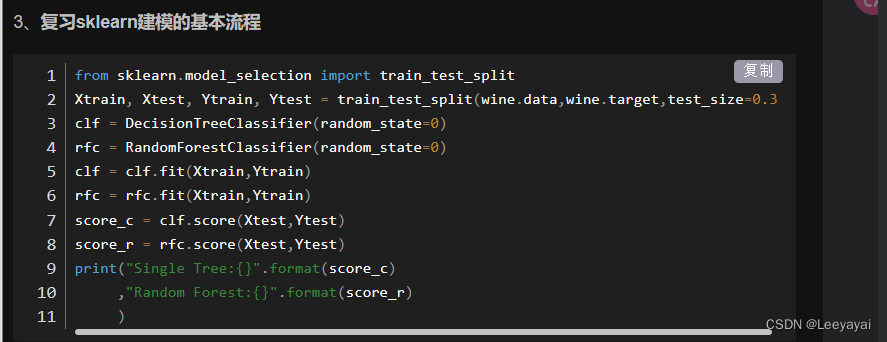
2:复习sklearn建模的基本流程
3: 建模与分析
画出随机森林和决策树在一组交叉验证下的效果对比
# 使用默认参数
model = RandomForestClassifier(oob_score=True, random_state=10)
model.fit(X_train,y_train)
test_predict = model.predict(X_test)from sklearn.metrics import accuracy_score
accuracy_score(y_test, test_predict)
0.6979166666666666
from sklearn.model_selection import cross_val_score
from sklearn.tree import DecisionTreeClassifier
from sklearn.ensemble import RandomForestClassifier
import matplotlib.pyplot as pltrfc = RandomForestClassifier(n_estimators=25)
rfc_s = cross_val_score(rfc,X_train,y_train,cv=10)
# 交叉验证划分为10折,
clf = DecisionTreeClassifier()
clf_s = cross_val_score(clf,X_train,y_train,cv=10)
plt.plot(range(1,11),rfc_s,label = "RandomForest")
plt.plot(range(1,11),clf_s,label = "Decision Tree")
plt.legend()
plt.show()
D:\anaconda\lib\site-packages\sklearn\model_selection\_split.py:676: UserWarning: The least populated class in y has only 8 members, which is less than n_splits=10.warnings.warn(
D:\anaconda\lib\site-packages\sklearn\model_selection\_split.py:676: UserWarning: The least populated class in y has only 8 members, which is less than n_splits=10.warnings.warn(

画出随机森林和决策树在10组交叉验证下的效果比较
rfc_l = []
clf_l = []
for i in range(10):rfc = RandomForestClassifier(n_estimators=25)rfc_s = cross_val_score(rfc,X_train,y_train,cv=10).mean()rfc_l.append(rfc_s)clf = DecisionTreeClassifier()clf_s = cross_val_score(clf,X_train,y_train,cv=10).mean()clf_l.append(clf_s)plt.plot(range(1,11),rfc_l,label = "Random Forest")
plt.plot(range(1,11),clf_l,label = "Decision Tree")
plt.legend()
plt.show()
#是否有注意到,单个决策树的波动轨迹和随机森林一致?
#再次验证了我们之前提到的,单个决策树的准确率越高,随机森林的准确率也会越高D:\anaconda\lib\site-packages\sklearn\model_selection\_split.py:676: UserWarning: The least populated class in y has only 8 members, which is less than n_splits=10.warnings.warn(
D:\anaconda\lib\site-packages\sklearn\model_selection\_split.py:676: UserWarning: The least populated class in y has only 8 members, which is less than n_splits=10.warnings.warn(
D:\anaconda\lib\site-packages\sklearn\model_selection\_split.py:676: UserWarning: The least populated class in y has only 8 members, which is less than n_splits=10.warnings.warn(
D:\anaconda\lib\site-packages\sklearn\model_selection\_split.py:676: UserWarning: The least populated class in y has only 8 members, which is less than n_splits=10.warnings.warn(
D:\anaconda\lib\site-packages\sklearn\model_selection\_split.py:676: UserWarning: The least populated class in y has only 8 members, which is less than n_splits=10.warnings.warn(
D:\anaconda\lib\site-packages\sklearn\model_selection\_split.py:676: UserWarning: The least populated class in y has only 8 members, which is less than n_splits=10.warnings.warn(
D:\anaconda\lib\site-packages\sklearn\model_selection\_split.py:676: UserWarning: The least populated class in y has only 8 members, which is less than n_splits=10.warnings.warn(
D:\anaconda\lib\site-packages\sklearn\model_selection\_split.py:676: UserWarning: The least populated class in y has only 8 members, which is less than n_splits=10.warnings.warn(
D:\anaconda\lib\site-packages\sklearn\model_selection\_split.py:676: UserWarning: The least populated class in y has only 8 members, which is less than n_splits=10.warnings.warn(
D:\anaconda\lib\site-packages\sklearn\model_selection\_split.py:676: UserWarning: The least populated class in y has only 8 members, which is less than n_splits=10.warnings.warn(
D:\anaconda\lib\site-packages\sklearn\model_selection\_split.py:676: UserWarning: The least populated class in y has only 8 members, which is less than n_splits=10.warnings.warn(
D:\anaconda\lib\site-packages\sklearn\model_selection\_split.py:676: UserWarning: The least populated class in y has only 8 members, which is less than n_splits=10.warnings.warn(
D:\anaconda\lib\site-packages\sklearn\model_selection\_split.py:676: UserWarning: The least populated class in y has only 8 members, which is less than n_splits=10.warnings.warn(
D:\anaconda\lib\site-packages\sklearn\model_selection\_split.py:676: UserWarning: The least populated class in y has only 8 members, which is less than n_splits=10.warnings.warn(
D:\anaconda\lib\site-packages\sklearn\model_selection\_split.py:676: UserWarning: The least populated class in y has only 8 members, which is less than n_splits=10.warnings.warn(
D:\anaconda\lib\site-packages\sklearn\model_selection\_split.py:676: UserWarning: The least populated class in y has only 8 members, which is less than n_splits=10.warnings.warn(
D:\anaconda\lib\site-packages\sklearn\model_selection\_split.py:676: UserWarning: The least populated class in y has only 8 members, which is less than n_splits=10.warnings.warn(
D:\anaconda\lib\site-packages\sklearn\model_selection\_split.py:676: UserWarning: The least populated class in y has only 8 members, which is less than n_splits=10.warnings.warn(
D:\anaconda\lib\site-packages\sklearn\model_selection\_split.py:676: UserWarning: The least populated class in y has only 8 members, which is less than n_splits=10.warnings.warn(
D:\anaconda\lib\site-packages\sklearn\model_selection\_split.py:676: UserWarning: The least populated class in y has only 8 members, which is less than n_splits=10.warnings.warn(

这篇关于葡萄酒数据集的随机森林分类的文章就介绍到这儿,希望我们推荐的文章对编程师们有所帮助!


