本文主要是介绍【AIGC】Diffusers:训练扩散模型,希望对大家解决编程问题提供一定的参考价值,需要的开发者们随着小编来一起学习吧!
前言
无条件图像生成是扩散模型的一种流行应用,它生成的图像看起来像用于训练的数据集中的图像。通常,通过在特定数据集上微调预训练模型来获得最佳结果。你可以在HUB找到很多这样的模型,但如果你找不到你喜欢的模型,你可以随时训练自己的模型!
本教程将教您如何在 Smithsonian Butterflies 数据集的子集上从头开始训练 UNet2DModel 以生成您自己的🦋蝴蝶🦋。
💡 本培训教程基于“扩散器训练🧨”笔记本。有关扩散模型的更多详细信息和背景信息,例如它们的工作原理,请查看笔记本!
在开始之前,请确保已安装 Datasets🤗 以加载和预处理图像数据集,并安装 Accelerate 🤗以简化任意数量的 GPU 上的训练。以下命令还将安装 TensorBoard 来可视化训练指标(您还可以使用权重和偏差来跟踪您的训练)。
# uncomment to install the necessary libraries in Colab
#!pip install diffusers[training]
我们鼓励您与社区分享您的模型,为此,您需要登录您的 Hugging Face 帐户(如果您还没有帐户,请在此处创建一个!您可以从笔记本登录,并在出现提示时输入您的令牌。确保您的令牌具有写入角色。
from huggingface_hub import notebook_loginnotebook_login()或从终端登录:
huggingface-cli login由于模型非常大,因此安装 Git-LFS 来对这些大文件进行版本控制:
!sudo apt -qq install git-lfs
!git config --global credential.helper store
训练配置
为方便起见,创建一个包含训练超参数的 TrainingConfig 类(随意调整它们):
from dataclasses import dataclass@dataclass
class TrainingConfig:image_size = 128  # the generated image resolutiontrain_batch_size = 16eval_batch_size = 16  # how many images to sample during evaluationnum_epochs = 50gradient_accumulation_steps = 1learning_rate = 1e-4lr_warmup_steps = 500save_image_epochs = 10save_model_epochs = 30mixed_precision = "fp16"  # `no` for float32, `fp16` for automatic mixed precisionoutput_dir = "ddpm-butterflies-128"  # the model name locally and on the HF Hubpush_to_hub = True  # whether to upload the saved model to the HF Hubhub_model_id = "<your-username>/<my-awesome-model>"  # the name of the repository to create on the HF Hubhub_private_repo = Falseoverwrite_output_dir = True  # overwrite the old model when re-running the notebookseed = 0config = TrainingConfig()
加载数据集
您可以使用 Datasets 🤗库轻松加载 Smithsonian Butterflies 数据集:
from datasets import load_datasetconfig.dataset_name = "huggan/smithsonian_butterflies_subset"
dataset = load_dataset(config.dataset_name, split="train")
💡 您可以从HugGan 社区活动中找到其他数据集,也可以通过创建本地 ImageFolder .如果数据集来自 HugGan 社区活动,或者 imagefolder 您使用的是自己的图像,请设置为 config.dataset_name 数据集的存储库 ID。
🤗 数据集使用Image功能自动解码图像数据并将其加载为 PIL.Image 我们可以可视化的:
import matplotlib.pyplot as pltfig, axs = plt.subplots(1, 4, figsize=(16, 4))
for i, image in enumerate(dataset[:4]["image"]):axs[i].imshow(image)axs[i].set_axis_off()
fig.show() 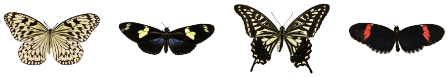
不过,这些图像的大小各不相同,因此您需要先对它们进行预处理:
Resize将图像大小更改为中config.image_size定义的大小。RandomHorizontalFlip通过随机镜像图像来扩充数据集。Normalize将像素值重新缩放到 [-1, 1] 范围非常重要,这是模型所期望的。
from torchvision import transformspreprocess = transforms.Compose([transforms.Resize((config.image_size, config.image_size)),transforms.RandomHorizontalFlip(),transforms.ToTensor(),transforms.Normalize([0.5], [0.5]),]
)
请随意再次可视化图像,以确认它们已调整大小。现在,您可以将数据集包装在 DataLoader 中进行训练了!
import torchtrain_dataloader = torch.utils.data.DataLoader(dataset, batch_size=config.train_batch_size, shuffle=True)创建 UNet2DModel
扩散器中的🧨预训练模型可以很容易地从其模型类中使用所需的参数创建。例如,若要创建 UNet2DModel:
from diffusers import UNet2DModelmodel = UNet2DModel(sample_size=config.image_size,  # the target image resolutionin_channels=3,  # the number of input channels, 3 for RGB imagesout_channels=3,  # the number of output channelslayers_per_block=2,  # how many ResNet layers to use per UNet blockblock_out_channels=(128, 128, 256, 256, 512, 512),  # the number of output channels for each UNet blockdown_block_types=("DownBlock2D",  # a regular ResNet downsampling block"DownBlock2D","DownBlock2D","DownBlock2D","AttnDownBlock2D",  # a ResNet downsampling block with spatial self-attention"DownBlock2D",),up_block_types=("UpBlock2D",  # a regular ResNet upsampling block"AttnUpBlock2D",  # a ResNet upsampling block with spatial self-attention"UpBlock2D","UpBlock2D","UpBlock2D","UpBlock2D",),
)
快速检查示例图像形状是否与模型输出形状匹配通常是一个好主意:
sample_image = dataset[0]["images"].unsqueeze(0)
print("Input shape:", sample_image.shape)print("Output shape:", model(sample_image, timestep=0).sample.shape)
接下来,您需要一个调度程序来向图像添加一些噪点。
创建调度程序
调度程序的行为会有所不同,具体取决于您是使用模型进行训练还是推理。在推理过程中,调度器会从噪声中生成图像。在训练过程中,调度器从扩散过程中的特定点获取模型输出或样本,并根据噪声调度和更新规则将噪声应用于图像。
让我们看一下DDPMScheduler 并使用该 add_noise 方法在 sample_image 前面添加一些随机噪声:
import torch
from PIL import Image
from diffusers import DDPMSchedulernoise_scheduler = DDPMScheduler(num_train_timesteps=1000)
noise = torch.randn(sample_image.shape)
timesteps = torch.LongTensor([50])
noisy_image = noise_scheduler.add_noise(sample_image, noise, timesteps)Image.fromarray(((noisy_image.permute(0, 2, 3, 1) + 1.0) * 127.5).type(torch.uint8).numpy()[0])该模型的训练目标是预测添加到图像中的噪声。这一步的损失可以通过以下方式计算:
import torch.nn.functional as Fnoise_pred = model(noisy_image, timesteps).sample
loss = F.mse_loss(noise_pred, noise)
训练模型
到现在为止,你已经有了开始训练模型的大部分,剩下的就是把所有东西放在一起。
首先,您需要一个优化器和一个学习率调度器:
from diffusers.optimization import get_cosine_schedule_with_warmupoptimizer = torch.optim.AdamW(model.parameters(), lr=config.learning_rate)
lr_scheduler = get_cosine_schedule_with_warmup(optimizer=optimizer,num_warmup_steps=config.lr_warmup_steps,num_training_steps=(len(train_dataloader) * config.num_epochs),
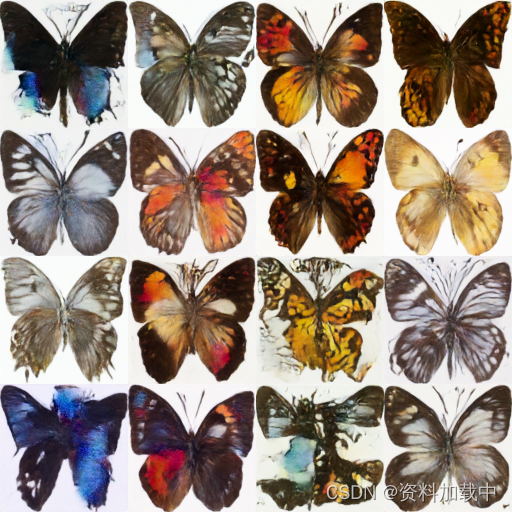
)然后,您需要一种方法来评估模型。为了进行评估,您可以使用 DDPMPipeline 生成一批示例图像并将其另存为网格:
from diffusers import DDPMPipeline
from diffusers.utils import make_image_grid
import osdef evaluate(config, epoch, pipeline):# Sample some images from random noise (this is the backward diffusion process).# The default pipeline output type is `List[PIL.Image]`images = pipeline(batch_size=config.eval_batch_size,generator=torch.manual_seed(config.seed),).images# Make a grid out of the imagesimage_grid = make_image_grid(images, rows=4, cols=4)# Save the imagestest_dir = os.path.join(config.output_dir, "samples")os.makedirs(test_dir, exist_ok=True)image_grid.save(f"{test_dir}/{epoch:04d}.png")
现在,您可以使用 Accelerate 将所有这些组件打包到训练循环🤗中,以便轻松进行 TensorBoard 日志记录、梯度累积和混合精度训练。若要将模型上传到 Hub,请编写一个函数来获取存储库名称和信息,然后将其推送到 Hub。
💡 下面的训练循环可能看起来令人生畏且漫长,但当您稍后仅用一行代码启动训练时,这将是值得的!如果您迫不及待地想要开始生成图像,请随时复制并运行下面的代码。您以后可以随时返回并更仔细地检查训练循环,例如在等待模型完成训练时。🤗
from accelerate import Accelerator
from huggingface_hub import create_repo, upload_folder
from tqdm.auto import tqdm
from pathlib import Path
import osdef train_loop(config, model, noise_scheduler, optimizer, train_dataloader, lr_scheduler):# Initialize accelerator and tensorboard loggingaccelerator = Accelerator(mixed_precision=config.mixed_precision,gradient_accumulation_steps=config.gradient_accumulation_steps,log_with="tensorboard",project_dir=os.path.join(config.output_dir, "logs"),)if accelerator.is_main_process:if config.output_dir is not None:os.makedirs(config.output_dir, exist_ok=True)if config.push_to_hub:repo_id = create_repo(repo_id=config.hub_model_id or Path(config.output_dir).name, exist_ok=True).repo_idaccelerator.init_trackers("train_example")# Prepare everything# There is no specific order to remember, you just need to unpack the# objects in the same order you gave them to the prepare method.model, optimizer, train_dataloader, lr_scheduler = accelerator.prepare(model, optimizer, train_dataloader, lr_scheduler)global_step = 0# Now you train the modelfor epoch in range(config.num_epochs):progress_bar = tqdm(total=len(train_dataloader), disable=not accelerator.is_local_main_process)progress_bar.set_description(f"Epoch {epoch}")for step, batch in enumerate(train_dataloader):clean_images = batch["images"]# Sample noise to add to the imagesnoise = torch.randn(clean_images.shape, device=clean_images.device)bs = clean_images.shape[0]# Sample a random timestep for each imagetimesteps = torch.randint(0, noise_scheduler.config.num_train_timesteps, (bs,), device=clean_images.device,dtype=torch.int64)# Add noise to the clean images according to the noise magnitude at each timestep# (this is the forward diffusion process)noisy_images = noise_scheduler.add_noise(clean_images, noise, timesteps)with accelerator.accumulate(model):# Predict the noise residualnoise_pred = model(noisy_images, timesteps, return_dict=False)[0]loss = F.mse_loss(noise_pred, noise)accelerator.backward(loss)accelerator.clip_grad_norm_(model.parameters(), 1.0)optimizer.step()lr_scheduler.step()optimizer.zero_grad()progress_bar.update(1)logs = {"loss": loss.detach().item(), "lr": lr_scheduler.get_last_lr()[0], "step": global_step}progress_bar.set_postfix(**logs)accelerator.log(logs, step=global_step)global_step += 1# After each epoch you optionally sample some demo images with evaluate() and save the modelif accelerator.is_main_process:pipeline = DDPMPipeline(unet=accelerator.unwrap_model(model), scheduler=noise_scheduler)if (epoch + 1) % config.save_image_epochs == 0 or epoch == config.num_epochs - 1:evaluate(config, epoch, pipeline)if (epoch + 1) % config.save_model_epochs == 0 or epoch == config.num_epochs - 1:if config.push_to_hub:upload_folder(repo_id=repo_id,folder_path=config.output_dir,commit_message=f"Epoch {epoch}",ignore_patterns=["step_*", "epoch_*"],)else:pipeline.save_pretrained(config.output_dir)
这可是一大堆代码啊!但是您终于可以使用 Accelerate 的notebook_launcher功能启动培训🤗了。向函数传递训练循环、所有训练参数和进程数(您可以将此值更改为可用的 GPU 数)以用于训练:
from accelerate import notebook_launcherargs = (config, model, noise_scheduler, optimizer, train_dataloader, lr_scheduler)notebook_launcher(train_loop, args, num_processes=1)训练完成后,查看扩散模型生成的最终🦋图像🦋!
import globsample_images = sorted(glob.glob(f"{config.output_dir}/samples/*.png"))
Image.open(sample_images[-1])
这篇关于【AIGC】Diffusers:训练扩散模型的文章就介绍到这儿,希望我们推荐的文章对编程师们有所帮助!


