智慧海洋建设-Task1地理数据分析常用工具

本文主要是介绍智慧海洋建设-Task1地理数据分析常用工具，希望对大家解决编程问题提供一定的参考价值，需要的开发者们随着小编来一起学习吧！

地理数据分析常用工具

安装geopandas的库时可以参考我的这篇文章《python库geopandas的安装方法》,https://blog.csdn.net/sjjsaaaa/article/details/115602267?utm_source=app&app_version=4.5.8

一.、shapely

Shapely是python中开源的空间几何对象库，支持Point、Curve和Surface等基本几何对象类型以及相关空间操作。另外，几何对象类型的特征分别有interior、boundary和exterior。

1.空间数据模型

1. point类型对应的方法在Point类中。curve类型对应的方法在LineString和LinearRing类中。surface类型对应的方法在Polygon类中。
2. point集合对应的方法在MultiPoint类中，curves集合对应的反方在MultiLineString类中，surface集合对应的方法在MultiPolygon类中。

2.几何对象的一些功能特性

• 几何对象可以和numpy.array互相转换。
• 可以求线的长度(length)，面的面积（area)，对象之间的距离(distance),最小最大距离(hausdorff_distance),对象的bounds数组(minx, miny, maxx, maxy)可以
• 求几何对象之间的关系：相交(intersect)，包含(contain)，求相交区域(intersection)等。
• 可以对几何对象求几何中心(centroid),缓冲区(buffer),最小旋转外接矩形(minimum_rotated_rectangle)等。
• 可以求线的插值点(interpolate),
• 可以求点投影到线的距离(project),
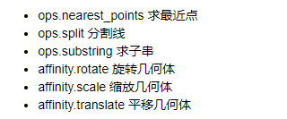
• 可以求几何对象之间对应的最近点(nearestPoint)
• 可以对几何对象进行旋转(rotate)和缩放(scale)

3.Point

from shapely import geometry as geo
from shapely import wkt 
from shapely import ops
import numpy as np 

赋值方式：

# point有三种赋值方式，具体如下
point = geo.Point(0.5,0.5)  
point_2 = geo.Point((0,0))  
point_3 = geo.Point(point)
# 其坐标可以通过coords或x，y，z得到
print(list(point_3.coords))
print(point_3.x)
print(point_3.y)
#批量进行可视化
geo.GeometryCollection([point,point_2])
print(np.array(point))#可以和np.array进行互相转换

4.LineStrings

几何对象的各种数值：

arr=np.array([(0,0), (1,1), (1,0)])
line = geo.LineString(arr) #等同于 line = geo.LineString([(0,0), (1,1), (1,0)]) print ('两个几何对象之间的距离:'+str(geo.Point(2,2).distance(line)))#该方法即可求线线距离也可以求线点距离
print ('两个几何对象之间的hausdorff_distance距离:'+str(geo.Point(2,2).hausdorff_distance(line)))#该方法求得是点与线的最长距离
print('该几何对象的面积:'+str(line.area))
print('该几何对象的坐标范围:'+str(line.bounds))
print('该几何对象的长度:'+str(line.length))
print('该几何对象的几何类型:'+str(line.geom_type))  
print('该几何对象的坐标系:'+str(list(line.coords)))
center = line.centroid #几何中心
geo.GeometryCollection([line,center])

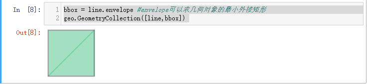
最小外接矩形

bbox = line.envelope #envelope可以求几何对象的最小外接矩形
geo.GeometryCollection([line,bbox]) 

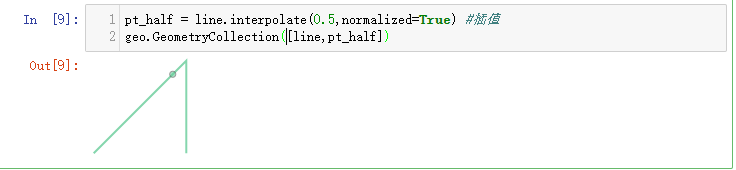
插值

pt_half = line.interpolate(0.5,normalized=True) #插值
geo.GeometryCollection([line,pt_half])

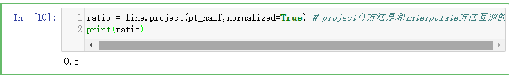
求值

ratio = line.project(pt_half,normalized=True) # project()方法是和interpolate方法互逆的
print(ratio)

5.DouglasPucker算法（轨迹分析中所用）

画出一条轨迹：

line1 = geo.LineString([(0,0),(1,-0.2),(2,0.3),(3,-0.5),(5,0.2),(7,0)])
line1_simplify = line1.simplify(0.4, preserve_topology=False)  #Douglas-Pucker算法
print(line1)
print(line1_simplify)
line1_simplify

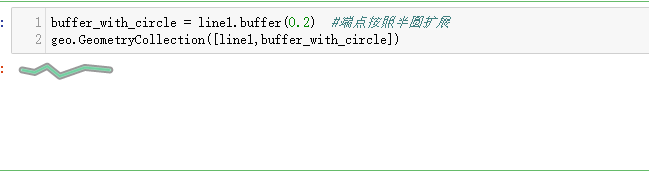
端点按照半圆扩展：

buffer_with_circle = line1.buffer(0.2)  #端点按照半圆扩展
geo.GeometryCollection([line1,buffer_with_circle])

6.LineRings

闭合图形：

# from shapely.geometry.polygon import LinearRing
ring = geo.polygon.LinearRing([(0, 0), (1, 1), (1, 0)])
print(ring.length)#相比于刚才的LineString的代码示例，其长度现在是3.41，是因为其序列是闭合的
print(ring.area)
geo.GeometryCollection([ring])

7.Polygon

组合图形：

from shapely.geometry import Polygon
polygon1 = Polygon([(0, 0), (1, 1), (1, 0)])
ext = [(0, 0), (0, 2), (2, 2), (2, 0), (0, 0)]
int = [(1, 0), (0.5, 0.5), (1, 1), (1.5, 0.5), (1, 0)]
polygon2 = Polygon(ext, [int])
print(polygon1.area)
print(polygon1.length)
print(polygon2.area)#其面积是ext的面积减去int的面积
print(polygon2.length)#其长度是ext的长度加上int的长度
print(np.array(polygon2.exterior))  #外围坐标点
geo.GeometryCollection([polygon2])

8.几何对象之间的关系

绘制凸包图形：

# 在下图中即为在给定6个point之后求其凸包，并绘制出来的凸包图形
points1 = geo.MultiPoint([(0, 0), (1, 1), (0, 2), (2, 2), (3, 1), (1, 0)])
hull1 = points1.convex_hull
geo.GeometryCollection([hull1,points1])

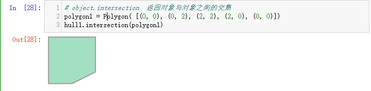
返回对象与对象之间的交集：

# object.intersection  返回对象与对象之间的交集
polygon1 = Polygon( [(0, 0), (0, 2), (2, 2), (2, 0), (0, 0)])
hull1.intersection(polygon1)

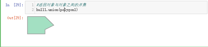
返回对象与对象之间的并集：

#返回对象与对象之间的并集
hull1.union(polygon1)

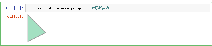
面面补集：

hull1.difference(polygon1) #面面补集

point、LineRing和LineString提供numpy数组接口，可以进行转换numpy数组

from shapely.geometry import asPoint,asLineString,asMultiPoint,asPolygon
import numpy as np
pa = asPoint(np.array([0.0, 0.0]))#将numpy数组转换成point格式
la = asLineString(np.array([[1.0, 2.0], [3.0, 4.0]]))#将numpy数组转换成LineString格式
ma = asMultiPoint(np.array([[1.1, 2.2], [3.3, 4.4], [5.5, 6.6]]))#将numpy数组转换成multipoint集合
pg = asPolygon(np.array([[1.1, 2.2], [3.3, 4.4], [5.5, 6.6]]))#将numpy数组转换成polygon
print(np.array(pa))#将Point转换成numpy格式

函数用法：

二、geopandas

• GeoPandas提供了地理空间数据的高级接口，它让使用python处理地理空间数据变得更容易。
• GeoPandas扩展了pandas。)使用的数据类型，允许对几何类型进行空间操作。几何运算由shapely执行。Geopandas进一步依赖fiona进行文件访问，依赖matplotlib进行绘图。

安装genpandas 可见——>https://blog.csdn.net/sjjsaaaa/article/details/115602267?spm=1001.2014.3001.5501

1.查看世界地图

import pandas as pd
import geopandas
import matplotlib.pyplot as plt
world = geopandas.read_file(geopandas.datasets.get_path('naturalearth_lowres'))#read_file方法可以读取shape文件，转化为GeoSeries和GeoDataFrame数据类型。
world.plot()#将GeoDataFrame变成图形展示出来，得到世界地图
plt.show()

查看geopandas ：world数据集：

2.绘制不同国家的人数

#根据每一个polygon的pop_est不同，便可以用python绘制图表显示不同国家的人数
fig, ax = plt.subplots(figsize=(9,6),dpi = 100)
world.plot('pop_est',ax = ax,legend = True)
plt.show()

三、Folium

folium可以满足我们平时常用的热力图、填充地图、路径图、散点标记等高频可视化场景.folium也可以通过flask让地图和我们的数据在网页上显示，极其便利。

1. 查看北京坐标地图

import folium
import os
#首先，创建一张指定中心坐标的地图，这里将其中心坐标设置为北京。zoom_start表示初始地图的缩放尺寸，数值越大放大程度越大
m=folium.Map(location=[39.9,116.4],zoom_start=10)
m

2.用Folium绘制热力图

import folium
import numpy as np
from folium.plugins import HeatMap
#先手动生成data数据，该数据格式由[纬度，经度，数值]构成
data=(np.random.normal(size=(100,3))*np.array([[1,1,1]])+np.array([[48,5,1]])).tolist()
# data

m=folium.Map([48,5],tiles='stamentoner',zoom_start=6)
HeatMap(data).add_to(m)
m 

3.参数

四、Kepler.gl

• Kepler.gl与folium类似，也是是一个图形化的数据可视化工具，基于Uber的大数据可视化开源项目deck.gl创建的demoapp。目前支持3种数据格式：CSV、JSON、GeoJSON。
• Kepler.gl提供了可视化图形案例，分别是Arc（弧）、Line（线）、Hexagon（六边形）、Point（点）、Heatmap（等高线图）、GeoJSON、Buildings（建筑）。

对智慧海洋题目进行数据处理

1.导入所需要的库

import pandas as pd 
import geopandas as gpd
from pyproj import Proj 
from keplergl import KeplerGl
from tqdm import tqdm
import os 
import matplotlib.pyplot as plt
import shapely
import numpy as np
from datetime import datetime  
import warnings
warnings.filterwarnings('ignore')
plt.rcParams['font.sans-serif'] = ['SimSun']    # 指定默认字体为新宋体。
plt.rcParams['axes.unicode_minus'] = False      # 解决保存图像时 负号'-' 显示为方块和报错的问题。

2.获取数据

定义获取数据的函数：

#获取文件夹中的数据
def get_data(file_path,model):assert model in ['train', 'test'], '{} Not Support this type of file'.format(model)paths = os.listdir(file_path)
#     print(len(paths))tmp = []for t in tqdm(range(len(paths))):p = paths[t]with open('{}/{}'.format(file_path, p), encoding='utf-8') as f:next(f)for line in f.readlines():tmp.append(line.strip().split(','))tmp_df = pd.DataFrame(tmp)if model == 'train':tmp_df.columns = ['ID', 'lat', 'lon', 'speed', 'direction', 'time', 'type']else:tmp_df['type'] = 'unknown'tmp_df.columns = ['ID', 'lat', 'lon', 'speed', 'direction', 'time', 'type']tmp_df['lat'] = tmp_df['lat'].astype(float)tmp_df['lon'] = tmp_df['lon'].astype(float)tmp_df['speed'] = tmp_df['speed'].astype(float)tmp_df['direction'] = tmp_df['direction'].astype(int)#如果该行代码运行失败，请尝试更新pandas的版本return tmp_df
# 平面坐标转经纬度，供初赛数据使用
# 选择标准为NAD83 / California zone 6 (ftUS) (EPSG:2230)，查询链接：https://mygeodata.cloud/cs2cs/
def transform_xy2lonlat(df):x = df['lat'].valuesy = df['lon'].valuesp=Proj('+proj=lcc +lat_1=33.88333333333333 +lat_2=32.78333333333333 +lat_0=32.16666666666666 +lon_0=-116.25 +x_0=2000000.0001016 +y_0=500000.0001016001 +datum=NAD83 +units=us-ft +no_defs ')df['lon'], df['lat'] = p(y, x, inverse=True)return df  
#修改数据的时间格式
def reformat_strtime(time_str=None, START_YEAR="2019"):"""Reformat the strtime with the form '08 14' to 'START_YEAR-08-14' """time_str_split = time_str.split(" ")time_str_reformat = START_YEAR + "-" + time_str_split[0][:2] + "-" + time_str_split[0][2:4]time_str_reformat = time_str_reformat + " " + time_str_split[1]
#     time_reformat=datetime.strptime(time_str_reformat,'%Y-%m-%d %H:%M:%S')return time_str_reformat
#计算两个点的距离
def haversine_np(lon1, lat1, lon2, lat2):lon1, lat1, lon2, lat2 = map(np.radians, [lon1, lat1, lon2, lat2])dlon = lon2 - lon1dlat = lat2 - lat1a = np.sin(dlat/2.0)**2 + np.cos(lat1) * np.cos(lat2) * np.sin(dlon/2.0)**2c = 2 * np.arcsin(np.sqrt(a))km = 6367 * creturn km * 1000def compute_traj_diff_time_distance(traj=None):"""Compute the sampling time and the coordinate distance."""# 计算时间的差值time_diff_array = (traj["time"].iloc[1:].reset_index(drop=True) - traj["time"].iloc[:-1].reset_index(drop=True)).dt.total_seconds() / 60# 计算坐标之间的距离dist_diff_array = haversine_np(traj["lon"].values[1:],  # lon_0traj["lat"].values[1:],  # lat_0traj["lon"].values[:-1], # lon_1traj["lat"].values[:-1]  # lat_1)# 填充第一个值time_diff_array = [time_diff_array.mean()] + time_diff_array.tolist()dist_diff_array = [dist_diff_array.mean()] + dist_diff_array.tolist()traj.loc[list(traj.index),'time_array'] = time_diff_arraytraj.loc[list(traj.index),'dist_array'] = dist_diff_arrayreturn traj #对轨迹进行异常点的剔除
def assign_traj_anomaly_points_nan(traj=None, speed_maximum=23,time_interval_maximum=200,coord_speed_maximum=700):"""Assign the anomaly points in traj to np.nan."""def thigma_data(data_y,n): data_x =[i for i in range(len(data_y))]ymean = np.mean(data_y)ystd = np.std(data_y)threshold1 = ymean - n * ystdthreshold2 = ymean + n * ystdjudge=[]for data in data_y:if (data < threshold1)|(data> threshold2):judge.append(True)else:judge.append(False)return judge# Step 1: The speed anomaly repairingis_speed_anomaly = (traj["speed"] > speed_maximum) | (traj["speed"] < 0)traj["speed"][is_speed_anomaly] = np.nan# Step 2: 根据距离和时间计算速度is_anomaly = np.array([False] * len(traj))traj["coord_speed"] = traj["dist_array"] / traj["time_array"]# Condition 1: 根据3-sigma算法剔除coord speed以及较大时间间隔的点is_anomaly_tmp = pd.Series(thigma_data(traj["time_array"],3)) | pd.Series(thigma_data(traj["coord_speed"],3))is_anomaly = is_anomaly | is_anomaly_tmpis_anomaly.index=traj.index# Condition 2: 轨迹点的3-sigma异常处理traj = traj[~is_anomaly].reset_index(drop=True)is_anomaly = np.array([False] * len(traj))if len(traj) != 0:lon_std, lon_mean = traj["lon"].std(), traj["lon"].mean()lat_std, lat_mean = traj["lat"].std(), traj["lat"].mean()lon_low, lon_high = lon_mean - 3 * lon_std, lon_mean + 3 * lon_stdlat_low, lat_high = lat_mean - 3 * lat_std, lat_mean + 3 * lat_stdis_anomaly = is_anomaly | (traj["lon"] > lon_high) | ((traj["lon"] < lon_low))is_anomaly = is_anomaly | (traj["lat"] > lat_high) | ((traj["lat"] < lat_low))traj = traj[~is_anomaly].reset_index(drop=True)return traj, [len(is_speed_anomaly) - len(traj)]

获取数据：

df=get_data(r'E:\Users\lenovo\Desktop\比赛学习实践练习合集\智慧海洋\数据\hy_round1_train_20200102','train')

3.对数据进行预处理

转换时间格式：

df=transform_xy2lonlat(df)
df['time']=df['time'].apply(reformat_strtime)
df['time']=df['time'].apply(lambda x: datetime.strptime(x,'%Y-%m-%d %H:%M:%S'))

对缺失值进行线性插值处理：

#对轨迹进行异常点剔除，对nan值进行线性插值
ID_list=list(pd.DataFrame(df['ID'].value_counts()).index)
DF_NEW=[]
Anomaly_count=[]
for ID in tqdm(ID_list):df_id=compute_traj_diff_time_distance(df[df['ID']==ID])df_new,count=assign_traj_anomaly_points_nan(df_id)df_new["speed"] = df_new["speed"].interpolate(method="linear", axis=0)df_new = df_new.fillna(method="bfill")df_new = df_new.fillna(method="ffill")df_new["speed"] = df_new["speed"].clip(0, 23)Anomaly_count.append(count)#统计每个id异常点的数量有多少DF_NEW.append(df_new)
DF=pd.concat(DF_NEW)

4.保存文件

DF=pd.read_csv('DF.csv')

5.数据查看

化简后的数据：

#douglas-peucker案例，由该案例可以看出针对相同ID的轨迹，可以先用geopandas将其进行简化和数据压缩
line= shapely.geometry.LineString(np.array(df[df['ID']=='11'][['lon','lat']]))
ax=gpd.GeoSeries([line]).plot(color='red')
ax = gpd.GeoSeries([line]).simplify(tolerance=0.000000001).plot(color='blue', ax=ax,linestyle='--')
LegendElement = [plt.Line2D([], [], color='red', label='简化前'),plt.Line2D([], [], color='blue', linestyle='--', label='简化后')]# 将制作好的图例映射对象列表导入legend()中，并配置相关参数
ax.legend(handles = LegendElement, loc='upper left', fontsize=10)
# ax.set_ylim((-2.1, 1))
# ax.axis('off')
print('化简前数据长度：'+str(len(np.array(gpd.GeoSeries([line])[0]))))
print('化简后数据长度：'+str(len(np.array(gpd.GeoSeries([line]).simplify(tolerance=0.000000001)[0]))))

6.转换格式

#定义数据简化函数。即通过shapely库将经纬度转换成LineString格式
#然后放入GeoSeries数据结构中并进行简化，最后再将所有数据放入GeoDataFrame中
def simplify_dataframe(df):line_list=[]for i in tqdm(dict(list(df.groupby('ID')))):line_dict={}lat_lon=dict(list(df.groupby('ID')))[i][['lon','lat']]line=shapely.geometry.LineString(np.array(lat_lon))line_dict['ID']=dict(list(df.groupby('ID')))[i].iloc[0]['ID']line_dict['type']=dict(list(df.groupby('ID')))[i].iloc[0]['type']  line_dict['geometry']=gpd.GeoSeries([line]).simplify(tolerance=0.000000001)[0]line_list.append(line_dict)return gpd.GeoDataFrame(line_list)

执行函数：

df_gpd_change=simplify_dataframe(DF)

需要六个小时才能跑完，谨慎跑！！！

导入功能模块：

df_gpd_change=pd.read_pickle('df_gpd_change.pkl') 

查看说明链接：

map1=KeplerGl(height=800)#zoom_start与这个height类似，表示地图的缩放程度
map1.add_data(data=df_gpd_change,name='data')
#当运行该代码后，下面会有一个kepler.gl使用说明的链接，可以根据该链接进行学习参考
map1

五、GeoHash

在对于经纬度进行数据分析和特征提取时常用到的是GeoHash编码，该编码方式可以将地理经纬度坐标编码为由字母和数字所构成的短字符串，它具有如下特性：

• 层级空间数据结构，将地理位置用矩形网格划分，同一网格内地理编码相同
• 只要编码长度足够长，可以表示任意精度的地理位置坐标
• 编码前缀匹配的越长，地理位置越邻近。

map1=KeplerGl(height=800)#zoom_start与这个height类似，表示地图的缩放程度
map1.add_data(data=DF,name='data')
#当运行该代码后，下面会有一个kepler.gl使用说明的链接，可以根据该链接进行学习参考
map1

IOPub data rate exceeded.
The notebook server will temporarily stop sending output
to the client in order to avoid crashing it.
To change this limit, set the config variable
--NotebookApp.iopub_data_rate_limit.
我的跑不动！！！！！！！
定义函数：

# reference: https://github.com/vinsci/geohash
def geohash_encode(latitude, longitude, precision=12):"""Encode a position given in float arguments latitude, longitude toa geohash which will have the character count precision."""lat_interval, lon_interval = (-90.0, 90.0), (-180.0, 180.0)base32 = '0123456789bcdefghjkmnpqrstuvwxyz'geohash = []bits = [16, 8, 4, 2, 1]bit = 0ch = 0even = Truewhile len(geohash) < precision:if even:mid = (lon_interval[0] + lon_interval[1]) / 2if longitude > mid:ch |= bits[bit]lon_interval = (mid, lon_interval[1])else:lon_interval = (lon_interval[0], mid)else:mid = (lat_interval[0] + lat_interval[1]) / 2if latitude > mid:ch |= bits[bit]lat_interval = (mid, lat_interval[1])else:lat_interval = (lat_interval[0], mid)even = not evenif bit < 4:bit += 1else:geohash += base32[ch]bit = 0ch = 0return ''.join(geohash)

调用函数：

#调用Geohash函数
DF[DF['ID']==1].apply(lambda x: geohash_encode(x['lat'], x['lon'], 7), axis=1)

GeoHash的主要价值在于将二维的经纬度坐标信息编码到了一维的字符串中，在做地理位置索引时只需要匹配字符串即可，便于缓存、信息压缩。在使用大数据工具（例如Spark）进行数据挖掘聚类时GeoHash显得更加便捷和高效。

这篇关于智慧海洋建设-Task1地理数据分析常用工具的文章就介绍到这儿，希望我们推荐的文章对编程师们有所帮助！

---