nlp-baseline 7：deep NMT

前言

本课程来自深度之眼deepshare.net，部分截图来自课程视频。
文章标题：Sequence to Sequence Learning with Neural Networks
使用多层LSTM的Seq2Seq模型/使用神经网络来做序列到序列的学习
作者：llya Sutskever，Oriol Vinyals，Quoc V. Le
单位：Google
发表会议及时间：NIPS2014
在线LaTeX公式编辑器
本文是大量实验中得到的一系列TRICK，提炼处理的文章，与普通的理论模型文章不太一样。

第一课 论文导读

a. 神经机器翻译概率
神经机器翻译就是使用神经网络使得机器能够自动将一种语言的句子翻译成另外一种语言的句子，它可以解决不同母语的人之间的交流障碍。
b. 两种神经机器翻译模型
最开始的神经机器翻译模型只是使用一个多层的LSTM，多层LSTM的最底层为源语言的输入，多层LSTM的最高层为目标语言的输出。之后产生了Encoder-Decoder的模型，即Encoder将源语言的句子压缩成一个向量，Decoder利用压缩得到的向量生成目标语言的句子。
c. LSTM以及多层LSTM
LSTM是一种特殊的RNN，通过增加一个记忆细胞和几个门来加强序列处理的长距离依赖。而多层LSTM就是单层LSTM网上叠加，上一层LSTM每一个时间步的输出作为当前层LSTM的输入。

BLEU介绍

BLEU 用来评价翻译的结果。
BLEU: a Method for Automatic Evaluation of Machine Translation, 2002
人工评价：通过人主观对翻译进行打分
优点：准确
缺点：速度慢，价格昂贵

机器自动评价：通过设置指标对翻译结果自动评价
优点：较为准确，速度快，免费
缺点：可能和人工评价有一些出入

BLEU实例

BLEU是一种评价指标，它可以用来自动对机器翻译的结果进行评价。
下面看一个BLEU评价的例子，假如我们现在有一句中文：
猫在垫上。
Candidate（翻译结果）: the the the the the the the.
Reference 1（参考答案1）: the cat is on the mat.
Reference 2（参考答案2）: there is a cat on the mat.
下面计算单词【the】出现在Candidate中的次数：
$$Count(the)=7Count(the)=7Count(the)=7$$
分别计算单词【the】出现在Reference 1和Reference 2中的次数：
$$\begin{gathered} Count1clip(the)=min(7,2)=2Count2clip(the)=min(7,1)=1Coun{t}_1^{clip}(the)=min(7,2)=2 \\ Coun{t}_2^{clip}(the)=min(7,1)=1Count1clip(the)=min(7,2)=2Count2clip(the)=min(7,1)=1 \end{gathered}$$
根据最大值得到单词【the】出现在参考答案中的次数：
$$Countclip(the)=max(2,1)=2Coun{t}^{clip}(the)=max(2,1)=2Countclip(the)=max(2,1)=2$$
最后计算出单词【the】BLEU：
$$p1=Countclip(the)Count(the)=2/7p_1=\frac{Coun{t}^{clip}(the)}{Count(the)}=2/7p1=Count(the)Countclip(the)=2/7$$
下标1代表1-gram
用代码表示：

from nltk.translate.bleu_score import sentence_bleu 
reference=[[' the',' cat',' is',' on',' the',' mat'],
[' there',' is','a',' cat',' on',' the',' mat']]
candidate=[' the',' the',' the',' the',' the',' the',' the']
score=sentence_bleu(reference, candidate, weights=(1,0,0,0))
# 这里的weights对应最终公式中的w，也就是每种gram的权重
print(score)

只计算1-gram，所以会有warning

BLEU改进

上面的例子可以看到，只考虑了1-gram的问题，这样的话，对每个词进行翻译就能得到很高的分，完全没考虑到句子的流利性。
改进：使用多-gram融合，如：使用1，2，3，4-gram。公式如下：
$$pn=\sum n-gram\in CCountclip(n-gram)\sum n-gram\in CCount(n-gram)p_n=\frac{{\sum }_{n-gram\in C}Coun{t}^{clip}(n-gram)}{{\sum }_{n-gram\in C}Count(n-gram)}pn=\sum n-gram\in CCount(n-gram)\sum n-gram\in CCountclip(n-gram)$$
还是上面的例子：
假如我们现在有一句中文：
猫在垫上。
Candidate（翻译结果）: the the the the the the the.
Reference 1（参考答案1）: the cat is on the mat.
Reference 2（参考答案2）: there is a cat on the mat.
在Candidate中的：
1-gram：the （在参考答案中出现的最大次数为2，$p1=2/7p_1=2/7p1=2/7$）
2-gram：the the （在参考答案中出现的最大次数为0，$p2=0p_2=0p2=0$）
3-gram：the the the （在参考答案中出现的最大次数为0，$p3=0p_3=0p3=0$）
4-gram：the the the the （在参考答案中出现的最大次数为0，$p4=0p_4=0p4=0$）
因此：
$$pn=0.25\times p1+0.25\times p2+0.25\times p3+0.25\times p4=1/14p_n=0.25\times p_1+0.25\times p_2+0.25\times p_3+0.25\times p_4=1/14pn=0.25\times p1+0.25\times p2+0.25\times p3+0.25\times p4=1/14$$
当然这样还是有问题，就是这个算法对于短句有利，例如：
假如我们现在有一句中文：
猫在垫上。
Candidate（翻译结果）: the.
Reference 1（参考答案1）: the cat is on the mat.
Reference 2（参考答案2）: there is a cat on the mat.
在Candidate中的：
1-gram：the （在参考答案中出现的最大次数为2，$p1=1/1p_1=1/1p1=1/1$）
2-gram：无 （在参考答案中出现的最大次数为0，$p2=0p_2=0p2=0$）
3-gram：无 （在参考答案中出现的最大次数为0，$p3=0p_3=0p3=0$）
4-gram：无 （在参考答案中出现的最大次数为0，$p4=0p_4=0p4=0$）
因此：
$$pn=0.25\times p1+0.25\times p2+0.25\times p3+0.25\times p4=1/4p_n=0.25\times p_1+0.25\times p_2+0.25\times p_3+0.25\times p_4=1/4pn=0.25\times p1+0.25\times p2+0.25\times p3+0.25\times p4=1/4$$
明显看到翻译结果还是很烂，但是句子变短以后分数变大了。
再次改进：对长度加上惩罚因子BP(BLEU punishment)。
KaTeX parse error: Expected '}', got 'EOF' at end of input: …(1−r/c) if c<r​
公式中r是Reference参考答案的长度，c是Candidate翻译结果的长度，从公式中可以看到当翻译结果的长度大于参考答案的长度，BP为1，不惩罚；当翻译结果的长度小于参考答案的长度时，$(1-r/c)<0,e(1-r/c)<1(1-r/c)<0,e^{(1-r/c)}<1(1-r/c)<0,e(1-r/c)<1$
平均指标BLEU公式变成：
$$BLEU=BP\cdot exp(\sum n=1Nwnlogpn)BLEU=BP\cdot \text{exp}\left(\sum _{n=1}^N{w}_n\text{log}{p}_n\right)BLEU=BP\cdot exp(n=1\sum Nwnlogpn)$$
这里用的是4-gram所以权重$wn{w}_{n}wn$有四个，分别对应1-gram到4-gram，这里还对$pn{p}_{n}pn$进行了log处理，log处理后大的会更大，接近0（越小）对应值越小。

机器翻译简介

机器翻译：使用机器自动将某种语言的一句话翻译成另外一种语言。
意义：可以解决人类之间因为不同语言交流不畅的问题。
16年的图：

机器翻译领域还有很多问题函待解决，19年ACL的BEST paper就是关于机器翻译中曝光度的研究。

机器翻译相关方法

Generating Sequences With Recurrent Neural Networks

加解码器来自下面的文章：
Learning Phrase Representations using RNN Encoder-Decoder for Statistical Machine Translation（好熟悉的文章名。。。）
Encoder：普通的LSTM，将一句话映射成一个向量C。
Decoder：对于隐藏层：
$$ht=f(ht-1,yt-1,c)h_t=f(h_{t-1},y_{t-1},c)ht=f(ht-1,yt-1,c)$$
对于输出层：
$$Pyt=g(ht,yt-1,c)P_{y_t}=g(h_t,y_{t-1},c)Pyt=g(ht,yt-1,c)$$

前期知识储备

·了解LSTM以及多层LSTM
·LSTM是最常用的RNN模型之一，RNN介绍可以参考
点我去看
·多层LSTM：实质上是单层LSTM的叠加
·了解Seq2Seq模型
·了解Seq2Seq模型的相关概念以及其中Encoder和Decoder的含义。可以参考点我去看

第二课 论文精读

论文整体框架

摘要

1. DNN在很多任务上取得了非常好的结果，但是它并不能解决Seq2Seq模型。Deep Neural Networks (DNNs) are powerful models that have achieved excellent performance on difficult learning tasks. Although DNNs work well whenever large labeled training sets are available, they cannot be used to map sequences to sequences.
2. 我们使用多层LSTM作为Encoder和Decoder，并且在WMT14英语到法语上取得了34.8的BLEU 的结果。In this paper, we present a general end-to-end approach to sequence learning that makes minimal assumptions on the sequence structure. Our method uses a multilayered Long Short-Term Memory (LSTM) to map the input sequence to a vector of a fixed dimensionality, and then another deep LSTM to decode the target sequence from the vector. Our main result is that on an English to French translation task from the WMT-14 dataset, the translations produced by the LSTM achieve a BLEU score of 34.8 on the entire test set, where the LSTM’s BLEU score was penalized on out-of-vocabulary words.
3. 此外，LSTM在长度上表现也很好，我们使用深度NMT模型来对统计机器翻译的结果进行重排序，能够使结果BLEU从33.3提高到36.5。Additionally, the LSTM did not have difficulty on long sentences. For comparison, a phrase-based SMT system achieves a BLEU score of 33.3 on the same dataset. When we used the LSTM to rerank the 1000 hypotheses produced by the aforementioned SMT system, its BLEU score increases to 36.5, which is close to the previous state of the art.
4. LSTM能够很好地学习到局部和全局的特征，最后我们发现对源句子倒序输入能够大大提高翻译的效果，因为这样可以缩短一些词从源语言到目标语言的依赖长度。t. The
   LSTM also learned sensible phrase and sentence representations that are sensitive to word order and are relatively invariant to the active and the passive voice. Finally, we found that reversing the order of the words in all source sentences (but not target sentences) improved the LSTM’s performance markedly, because doing so introduced many short term dependencies between the source and the target sentence which made the optimization problem easier.

1.介绍

1. 深度神经网络非常成功，但是却很难处理序列到序列的问题。
2. 本文使用一种新的Seq2Seq模型结果来解决序列到序列的问题，其中Seq2Seq模型的Encoder
   和Decoder都使用的是LSTM。
3. 前人研究者针对这个问题已经有了很多工作，包括Seq2Seq模型和注意力机制。
4. 本文的深度Seq2Seq模型在机器翻译上取得了非常好的效果。

2.模型
3.实验
4相关工作
5&6.总结&致谢

1. Introduction
2. The Model
3. Experiments
   3.1 Dataset details
   3.2 Decoding and Rescoring
   3.3 Reversing the Source Sentences
   3.4 Training details
   3.5 Parallelization
   3.6 Experimental Results
   3.7 Performance on long sentences
   3.8 Model Analysis
4. Related Work
5. Conclusion

传统/经典算法模型

1.Encoder-Decoder(见导读)

2.基于attention的机器翻译

来自之前读过的：Neural Machine Translation by Jointly Learning to Align and Translate
Encoder：单层双向LSTM。(就是下图中下面两层方框)
Decoder：
对于输出：
$$p(yi)=g(yi-1,si,ci)p(y_i)=g(y_{i-1},s_i,c_i)p(yi)=g(yi-1,si,ci)$$
对于$ci{c}_{i}ci$：
$$ci=\sum j=1Txaijhj,aij=exp(eij)\sum k=1Txexp(eik)c_i=\sum _{j=1}^{T_x}{a}_{ij}{h}_j,a_{ij}=\frac{exp(e_{ij})}{{\sum }_{k=1}^{T_x}exp(e_{ik})}ci=j=1\sum Txaijhj,aij=\sum k=1Txexp(eik)exp(eij)$$
$$whereeij=a(sj-1,hj)where{e}_{ij}=a(s_{j-1},h_j)whereeij=a(sj-1,hj)$$

本文模型

深度神经机器翻译模型Deep Neural Machine Translation Model，Deep NMT模型
1.Encoder和Decoder是不同的LSTM。（下图中有白色Encoder和黄色Decoder）不同颜色的的两个LSTM之间参数当然不共享
2.使用4层的深度LSTM。（从下往上数）隐层参数以白色那个为例应该是：
$$h14h24h34h13h23h33h12h22h32h11h21h31\begin{array}{ccc}{h}_1^4& h_2^4& h_3^4\\ h_1^3& h_2^3& h_3^3\\ h_1^2& h_2^2& h_3^2\\ h_1^1& h_2^1& h_3^1\end{array}h14h13h12h11h24h23h22h21h34h33h32h31$$
白色Encoder和黄色Decoder的参数是同时训练的。
3.将输入逆序输入。（原输入是ABC）这样输入的开始部分和输出离得比较近，因此开始部分翻译效果比较好，但是会导致后面部分翻译效果一般。

4.最下面那里的黄色的输入是训练的时候才有的。
5.本文算法里面貌似还用到了维特比和Beam Search，不展开写。

Tricks

1. 对于Encoder和Deocder，使用不同的LSTM。
2. 深层的LSTM比浅层的LSTM效果好。（当然也不能太深，太深不好训练，也容易梯度消失）
3. 对源语言倒序输入（Reverse the order）会大幅度提高翻译效果。
4. 对句子划分batch之前按长度进行排序，避免了大量的由于长句产生的pad，将速度提高了2倍

应用

1. 是谷歌翻译的基础。就是后面的GNMT
2. 多层的LSTM配合Attention是Transformer出来前最好的模型。

实验和结果

数据集

WMT’14English to French：包含36M英语到法语的双语语料，是机器翻译领域最常用的语料之一。
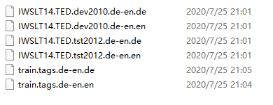
lwslt14English to German：包含170K英语到德语的双语语料，机器翻译领域最常用的语料之一，是一个相对较小的语料。（这个能跑）

数据集中语料是英文和德文个一个
各取前4句看看：

<url>http://www.ted.com/talks/stephen_palumbi_following_the_mercury_trail.html</url>
It can be a very complicated thing, the ocean.
And it can be a very complicated thing, what human health is.
And bringing those two together might seem a very daunting task, but what I'm going to try to say is that even in that complexity, there's some simple themes that I think, if we understand, we can really move forward.
And those simple themes aren't really themes about the complex science of what's going on, but things that we all pretty well know.

<url>http://www.ted.com/talks/lang/de/stephen_palumbi_following_the_mercury_trail.html</url>
Das Meer kann ziemlich kompliziert sein.
Und was menschliche Gesundheit ist, kann auch ziemlich kompliziert sein.
Und diese zwei zusammen zu bringen, erscheint vielleicht wie eine gewaltige Aufgabe. Aber was ich Ihnen zu sagen versuche ist, dass es trotz dieser Komplexität einige einfache Themen gibt, von denen ich denke, wenn wir diese verstehen, können wir uns wirklich weiter entwickeln.
Und diese einfachen Themen sind eigentlich keine komplexen wissenschaftlichen Zusammenhänge, sondern Tatsachen,die wir alle gut kennen.

实验结果

Deep NMT直接和baseline模型的对比。
本文提出的模型在单模型上比Bahdanau的基于attention的模型（第一个）要好得多，并且继承多个模型之后得到了非常好的结果。
single代表单个模型，不是单层LSTM。
这里用到了Beam Search，每个分支保留1个结果，到每个分支保留2个结果时，得分增加比较明显（从33.00到34.50），再增加到每个分支12个结果，效果没有这么明显（从34.50到34.81）。

使用本文提出的模型结合统计机器翻译模型（具体就是对机器翻译的结果进行重新打分，排序），最终得到了比state-of-the-art只差0.5的相当好的结果。
关于打分原文是：
We also used the LSTM to rescore the 1000-best lists produced by the baseline system [29]. To rescore an n-best list, we computed the log probability of every hypothesis with our LSTM and took an even average with their score and the LSTM’s score.
意思就是用统计机器翻译（SMT）的得分与本文模型得分进行平均，然后结果排序，选最好那个。

该模型对词序是敏感的（以下几个图是通过PCA对8000维的词表示进行降维得到的二维结果）：

对于主动和被动语态也分得很清楚：

翻译结果和长度（左边）以及词频（右边）的关系。

讨论和总结

讨论

为什么要讲这篇论文？
这篇论文提出的多层LSTM的结构是transformer出来之前机器翻译领域的标准做法。
本文提出的模型有何缺点？
LSTM的缺点就是并行差，所以后来有很多使用CNN和transformer做机器翻译的文章。
后来的改进模型？
后来的改进主要集中在attention上。

总结（主要创新点）

A.对于Encoder和Decoder使用不同的LSTM。
B.在Encoder和Decoder中都是用了多层LSTM。
C.对输入进行逆序输入可以大大提高翻译效果。

对比模型：本文对比了基于attention的神经机器翻译模型和传统的统计机器翻译模型。
模型：本文提出了一种基于多层LSTM的神经机器翻译模型。
实验：本文提出的模型在单模型和结合统计机器翻译的模型上都取得了非常好的结果。

关键点
• 验证了Seq2Seq模型对于序列到序列任务的有效性。
• 从实验的角度发现了很多提高翻译效果的tricks
• Deep NMT模型
创新点
• 提出了一种新的神经机器翻译模型—Deep NMT模型
• 提出了一些提高神经机器翻译效果的tricks——多层LSTM和倒序输入等。
• 在WMT14英语到法语翻译上得到了非常好的结果。

启发点
• Seq2Seq模型就是使用一个LSTM提取输入序列的特征，每个时间步输入一个词，从而生成固定维度的句子向量表示，然后Deocder使用另外一个LSTM来从这个向量中生成输入序列。
The idea is to use one LSTM to read the input sequence, one timestep at a time, to obtain large fixed dimensional vector representation, and then to use another LSTM to extract the output sequence
from that vector(Introduction P3)

这里的Encoder和Decoder的思想非常重要，这里是用LSTM来作为Encoder和Decoder，后面还出现了CNN，RNN作为Encoder和Decoder的文章。

• 我们的实验也支持这个结论，我们的模型生成的句子表示能够明确词序信息，并且能够识别出来同一 种含义的主动和被动语态。
A qualitative evaluation supports this claim, showing that our model is aware of word order and is fairly invariant to the active and passive voice.(Introduction P8)

参考论文

D. Bahdanau,K. Cho, and Y. Bengio. Neural machine translation by jointly learning to align and translate. arXiv preprint arXiv:1409.0473,2014.

代码复现

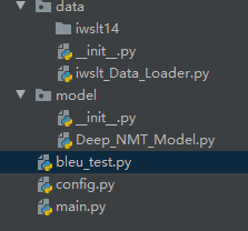
代码结构

数据集

IWSLT14
19M左右
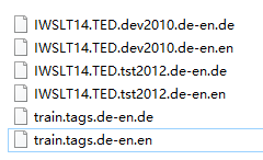
原始数据中有xml格式的，要预先处理。
弄成这样

在训练集里面还有一些网站url标签，读取的时候要过滤掉
最后的训练数据大概16w条
载入数据集后打印第一条的
print(iwslt_data.source_data[0])#反向之后pad之后的0在前面了
print(iwslt_data.target_data_input[0])#以"": 2开头
print(iwslt_data.target_data[0])#以"": 3结尾

数据处理

这里是要读取源语言和目标语言，所以处理两种语言代码有部分不一样，要分开写，具体看注释

作业

多层LSTM为什么比单层LSTM要好，对输入逆序为什么能够提高效果，试分析原因？
答：这里的多层LSTM是指垂直方向的堆叠，横向的是不同时间步（sequence or timestep）的堆叠。多层LSTM从模型的复杂度的角度上来看，肯定要比单层的LSTM模型要复杂，从理论上来说，越复杂的模型其涵盖的特征空间就越大，也就是可以用来获取或者表达越复杂的特征。一个简单的例子就是，一条直线（线性模型），只能把平面粗暴划分成两类，但是如果二次方程可以拟合出复杂些的曲线。关于为什么要进行深度或者说多层的叠加，可以参考李宏毅老师Why Deep(上)和Why Deep(下)。
但是从实作上面来看，不可能无限的加深，因为会有梯度消失和梯度爆炸等问题困扰，当然为了解决这些问题，有残差网络、梯度cliff等思想的提出，但是计算能力以及训练难度也是拦路虎，越复杂的模型计算能力要求越高，训练数据要求越多。
关于词的逆序输入问题，原文已经解释很清楚了，因此大量的句子进行输入的时候，后面是pad进行补齐到指定长度的，因此都是数据在前，屁股后面一堆0的情况，而最终Encoder得到的向量和距离它最近的层相关性会比较强，我们把输入数据反序后，0在前，数据靠后，就使得数据接近Encoder得到的向量，效果自然有变好。不知道Bi-LSTM是不是也是解决这个问题的方法之一。