[环境保护探索]-对水资源可饮用程度的数据探索性分析及预测

---

项目背景

数据集题材： [环境保护探索] 饮用水资源的可用性分析

数据集形式： csv文本格式，数据源自Kaggle。共 32760 条数据，以及 10 个原始特征和标签 (3276 X 10)

项目数据探索目的(译自原文)：

获得安全饮用水对健康至关重要，既是一项基本人权，也是一个重要的经济发展问题。在一些地区已经表明，对供水和卫生设施的投资可以产生净经济效益。

本项目旨在对水资源数据的9项水质指标展开探索分析，以及构造模型预测的水体可饮用性，为水资源的保护和合理开发提供数据支持与决策。

水质指标：

pH值(ph)：评价水的酸碱平衡的一个重要参数，世卫建议pH值的最大允许限值为6.5至8.5

硬度(Hardness)：硬度主要由钙和镁盐引起，被定义为水沉淀钙镁引起的凝块沉淀的容度

总溶解固体(Solids)：TDS值较高的水表明该水具有较高的矿化度。TDS的理想限值为500 mg/l，最大限值为1000 mg/l，规定用于饮用

氯胺(Chloramines)： 氯和氯胺是公共供水系统中使用的主要消毒剂，饮用水中氯含量高达4毫克/升被认为是安全的。

硫酸盐(Sulfate)：化学工业污染物，在大多数淡水供应中，其浓度范围为3至30毫克/升

电导率(Conductivity)：水中溶解固体的数量决定电导率，世卫标准，EC值不应超过400μS/cm

有机碳(Organic_carbon)：对纯净水中有机化合物中碳总量的测量。美国环保局规定，经处理/饮用水中的TOC<2 mg/L，用于处理的水源水中的TOC<4 mg/L

三卤甲烷(Trihalomethanes)：三卤甲烷可能存在于经过氯处理的水中，饮用水中THM含量高达80 ppm被认为是安全的

浊度(Turbidity)：水的浊度取决于悬浮状态下存在的固体物质的数量。世界卫生组织建议值5.00 NTU

---

可饮用性(Potability)：表示水对人类饮用是否安全，其中1表示饮用水，0表示不饮用水。

一、数据导入、简单预览，以及预处理

1.引入库

# 通用模块
import pandas as pd
import matplotlib.pyplot as plt
import seaborn as sns
import numpy as np
import plotly.express as px
from collections import Counter
import matplotlib
zhfont1 = matplotlib.font_manager.FontProperties(fname="SourceHanSansSC-Bold.otf")
from warnings import filterwarnings
# 机器学习
from sklearn.model_selection import train_test_split, KFold, cross_validate, cross_val_score
from sklearn.preprocessing import StandardScaler,MinMaxScaler
from sklearn.linear_model import LogisticRegression,RidgeClassifier,SGDClassifier,PassiveAggressiveClassifier
from sklearn.linear_model import Perceptron
from sklearn.svm import SVC,LinearSVC,NuSVC
from sklearn.neighbors import KNeighborsClassifier,NearestCentroid
from sklearn.tree import DecisionTreeClassifier
from sklearn.ensemble import RandomForestClassifier,AdaBoostClassifier,GradientBoostingClassifier
from sklearn.svm import SVC
from sklearn.naive_bayes import GaussianNB,BernoulliNB
from sklearn.ensemble import VotingClassifier
from sklearn.metrics import precision_score,accuracy_score
from sklearn.model_selection import RandomizedSearchCV,GridSearchCV,RepeatedStratifiedKFold
from sklearn.metrics import accuracy_score

2.读入数据

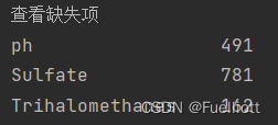
 data = pd.read_csv(r'C:\xlwings\water\water_potability.csv')  # 导入数据print('预览数据')print(data.head(3).T)  # 预览数据print('查看各字段属性')  # 查看各字段属性print(data.info())print('查看缺失项')  # 查看缺失项print(data.isnull().sum()[data.isnull().sum().values != 0].T)  # 得出children,country,agent,company四个字段含有缺失项# msno.bar(data, figsize=(10, 7), fontsize=10, color='grey',log=True)  # log=True 切换到对数刻度,更为清晰# plt.show()print('查看数据大小')  # 查看数据大小print(data.size)print(data.shape)print('看数据数据及分布')  # 查看数据数据及分布print(data.describe().T)

---

结果：
1.共 32760 条数据，以及 10 个原始特征和标签 (3276 X 10)
2.缺失项：

3.处理缺失值

    d1=data[data['Potability'] == 0][['ph', 'Sulfate', 'Trihalomethanes']].median()d2=data[data['Potability'] == 1][['ph', 'Sulfate', 'Trihalomethanes']].median()d=pd.DataFrame({'Potability=0':d1,'Potability=1':d2})   #查看中值差异print('查看中值差异')print(d)e1=data[data['Potability'] == 0][['ph', 'Sulfate', 'Trihalomethanes']].mean()e2 = data[data['Potability'] == 1][['ph', 'Sulfate', 'Trihalomethanes']].mean()e=pd.DataFrame({'Potability=0':e1,'Potability=1':e2})print(e)print('结论：经过对比，饮用水和非饮用水数据中各自关于ph、Sulfate、Trihalomethanes的均值和中位数差异都不大，因此选择中位数作为缺失项的填充值。')

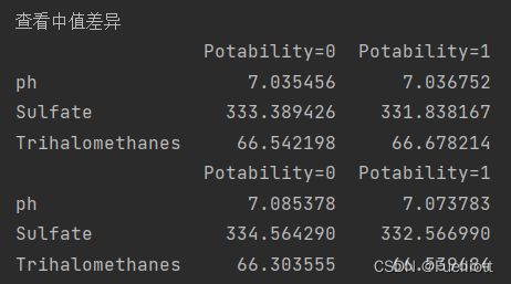
结论：经过对比，饮用水和非饮用水数据中各自关于ph、Sulfate、Trihalomethanes的均值和中位数差异都不大，因此选择中位数作为缺失项的填充值。

3.1填充缺失值：

data['ph'].fillna(value=data['ph'].median(), inplace=True)
data['Sulfate'].fillna(value=data['Sulfate'].median(), inplace=True)
data['Trihalomethanes'].fillna(value=data['Trihalomethanes'].median(), inplace=True)
print(data.isnull().sum())  # 缺失值全部被填充data.to_csv(r'C:\xlwings\water\water_potability_full.csv')
print('输出处理后的数据集')

二、水质指标的数据分析

1.各水质特征的数据分布

1.1 硬度

    def pic_hardness():fig = px.histogram(data_full, x='Hardness', y=Counter(data_full['Hardness']), color='Potability', template='plotly_white',marginal='box', opacity=0.7, nbins=100,color_discrete_sequence=[colors_green[3], colors_blue[3]],barmode='group', histfunc='count')           #作直方图  边际画箱型图  marginal=`rug`、`box`, `violin`fig.add_vline(x=151, line_width=1, line_color=colors_dark[1], line_dash='dot', opacity=0.7)fig.add_vline(x=301, line_width=1, line_color=colors_dark[1], line_dash='dot', opacity=0.7)fig.add_vline(x=76, line_width=1, line_color=colors_dark[1], line_dash='dot', opacity=0.7)fig.add_annotation(text='<76 mg/L <br> 被视作软水', x=40, y=130, showarrow=False, font_size=9)fig.add_annotation(text=' 76 ~150<br> (mg/L) 之间<br>被视作中等硬度', x=113, y=130, showarrow=False,font_size=9)fig.add_annotation(text='151 ~300 (mg/L)<br> 之间<br>被视作硬水', x=250, y=130, showarrow=False,font_size=9)fig.add_annotation(text='>300 mg/L<br> 被视作水质非常硬', x=340, y=130, showarrow=False, font_size=9)fig.update_layout(font_family='monospace',title=dict(text='水质硬度分布图', x=0.53, y=0.95,font=dict(color=colors_dark[2], size=20)),xaxis_title_text='Hardness (mg/L)',yaxis_title=dict(text='计数'),legend=dict(x=1, y=0.96, bordercolor=colors_dark[4], borderwidth=0, tracegroupgap=5),bargap=0.3,)fig.show()'硬水占比'print(data_full['Hardness'[data_full['Hardness']>151].count()/data_full['Hardness'].count())return# pic_hardness()

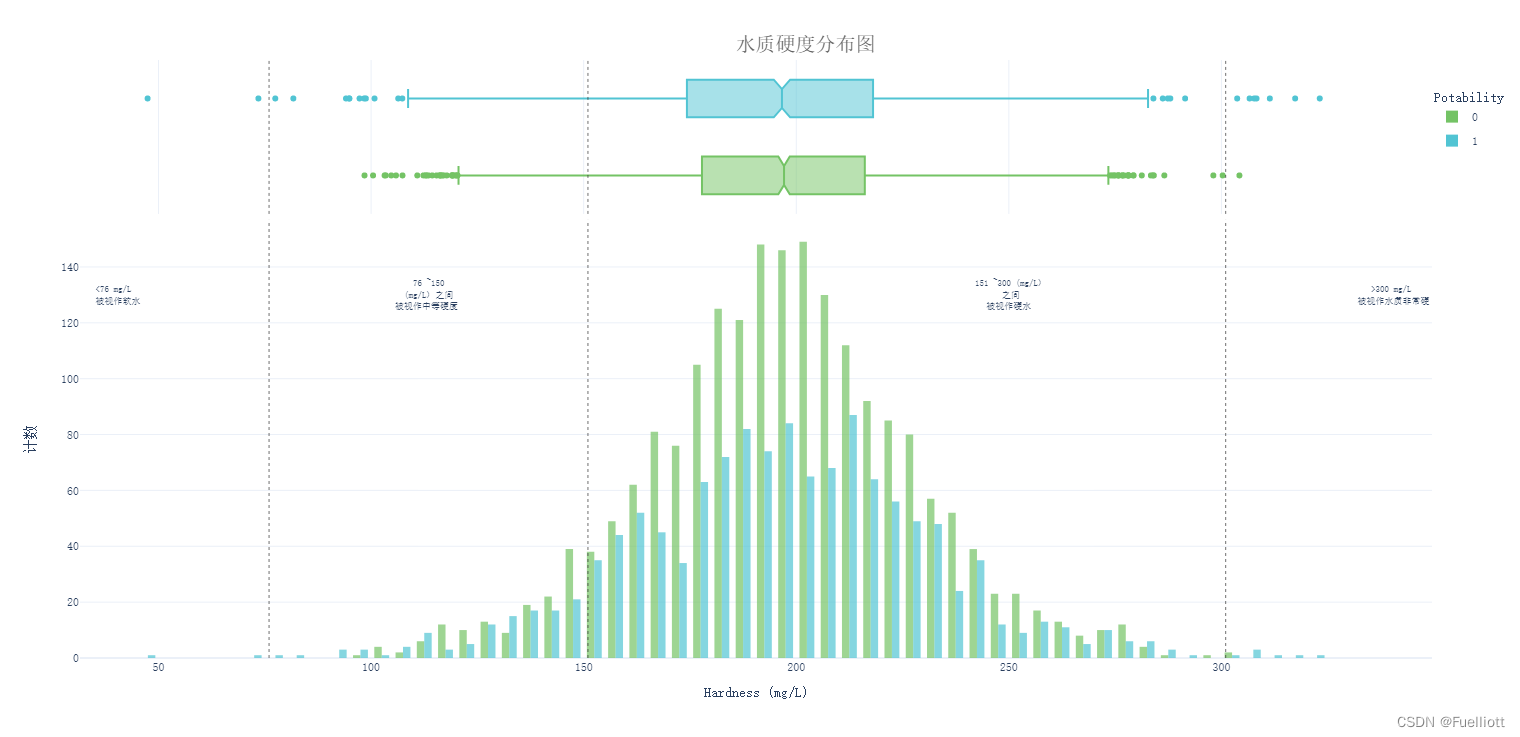
结论：数据集中92%的水质样本属于硬水性质。

1.2 PH值

    def pic_ph():fig = px.histogram(data_full, x='ph',y=data_full['ph'], color='Potability', template='plotly_white',marginal='box', opacity=0.7, nbins=100,color_discrete_sequence=[colors_green[3], colors_blue[3]],barmode='group', histfunc='count')fig.add_vline(x=7, line_width=1, line_color=colors_dark[1], line_dash='dot', opacity=0.7)fig.add_annotation(text='<7 呈酸性', x=4, y=70, showarrow=False, font_size=10)fig.add_annotation(text='>7 呈碱性', x=10, y=70, showarrow=False, font_size=10)fig.update_layout(font_family='monospace',title=dict(text='pH 值分布图', x=0.5, y=0.95,font=dict(color=colors_dark[2], size=20)),xaxis_title_text='pH Level',yaxis_title_text='Count',legend=dict(x=1, y=0.96, bordercolor=colors_dark[4], borderwidth=0, tracegroupgap=5),bargap=0.3,)fig.show()return# pic_ph()

结论：数据种包含的酸性和碱性pH值水样数量几乎相等。

1.3总溶解固体-TDS

def pic_solids():fig = px.histogram(data_full, x='Solids', color='Potability', template='plotly_white',marginal='box', opacity=0.7, nbins=100,color_discrete_sequence=[colors_green[3], colors_blue[3]],barmode='group', histfunc='count')fig.update_layout(font_family='monospace',title=dict(text='总溶解固体分布图', x=0.5, y=0.95,font=dict(color=colors_dark[2], size=20)),xaxis_title_text='Dissolved Solids (ppm)',yaxis_title_text='Count',legend=dict(x=1, y=0.96, bordercolor=colors_dark[4], borderwidth=0, tracegroupgap=5),bargap=0.3,)fig.show()# pic_solids()

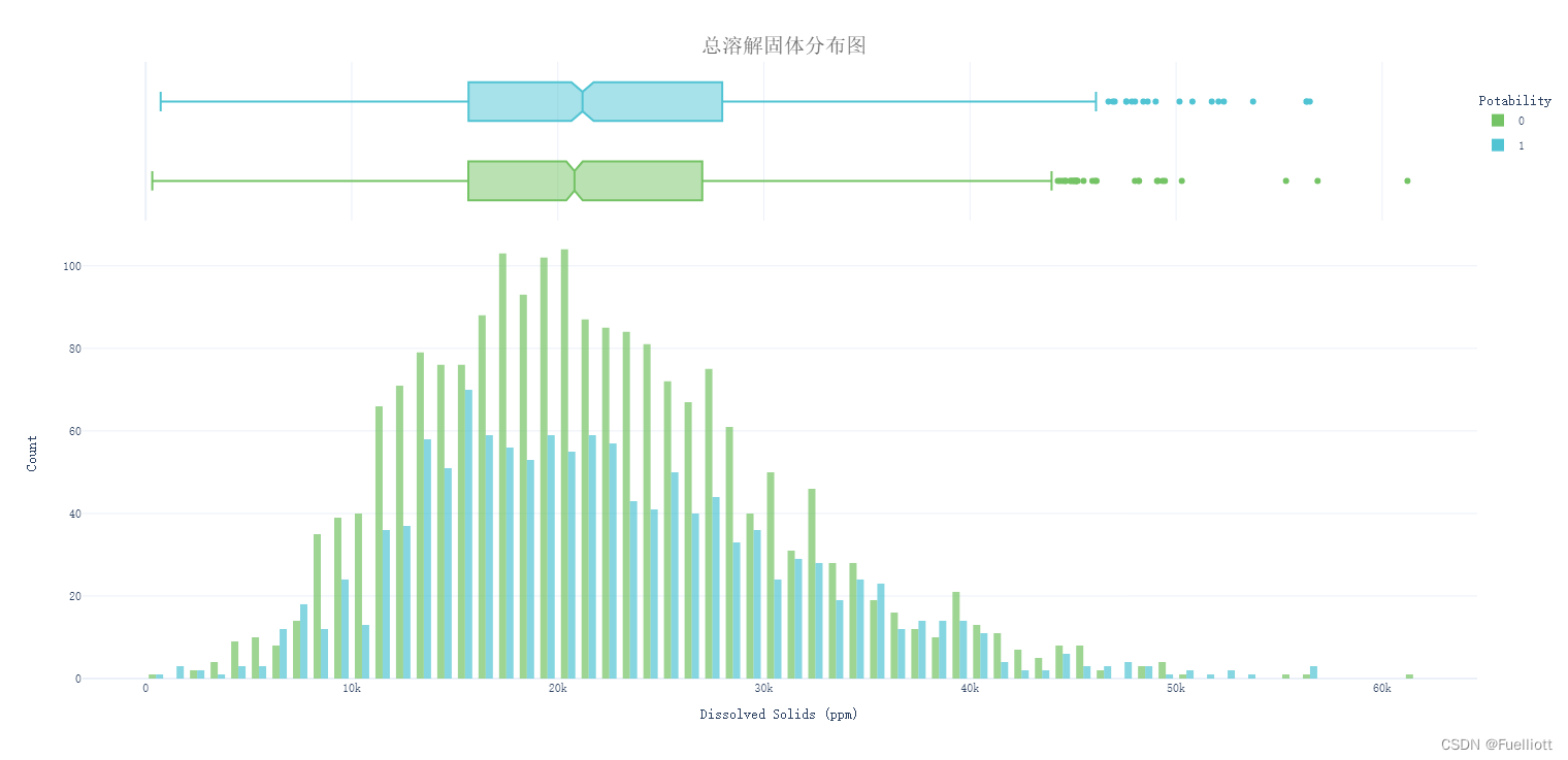
结论：可饮用水的理想TDS最大限值为1000 mg/l，数据样本中绝大多数的TDS值都超标了20到40倍，存在数据单位差异的可能性，需要进一步探究。

1.4氯胺

    def pic_Chloramines():fig = px.histogram(data_full, x='Chloramines', color='Potability',template='plotly_white',marginal='box', opacity=0.7, nbins=100,color_discrete_sequence=[colors_green[3], colors_blue[3]],barmode='group', histfunc='count')fig.add_vline(x=4, line_width=1, line_color=colors_dark[1], line_dash='dot', opacity=0.7)fig.add_annotation(text='<4 ppm 被视作<br> 可安全饮用', x=1.8, y=90, showarrow=False)fig.update_layout(font_family='monospace',title=dict(text='氯胺含量分布', x=0.53, y=0.95,font=dict(color=colors_dark[2], size=20)),xaxis_title_text='Chloramines (ppm)',yaxis_title_text='Count',legend=dict(x=1, y=0.96, bordercolor=colors_dark[4], borderwidth=0, tracegroupgap=5),bargap=0.3,)fig.show()return# pic_Chloramines()

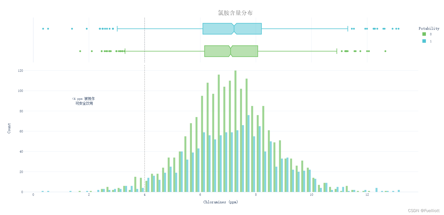
结论：就氯胺水平而言，只有2%的水样是可以安全饮用的。

1.5硫酸盐

    def pic_Sulfate():fig = px.histogram(data_full, x='Sulfate',color='Potability', template='plotly_white',marginal='box', opacity=0.7, nbins=100,color_discrete_sequence=[colors_green[3], colors_blue[3]],barmode='group', histfunc='count')fig.add_vline(x=250, line_width=1, line_color=colors_dark[1], line_dash='dot', opacity=0.7)fig.add_annotation(text='<250 mg/L 被视作<br> 可安全饮用', x=175, y=90, showarrow=False)fig.update_layout(font_family='monospace',title=dict(text='硫酸盐含量分布', x=0.53, y=0.95,font=dict(color=colors_dark[2], size=20)),xaxis_title_text='Sulfate (mg/L)',yaxis_title_text='Count',legend=dict(x=1, y=0.96, bordercolor=colors_dark[4], borderwidth=0, tracegroupgap=5),bargap=0.3,)fig.show()return# pic_Sulfate()

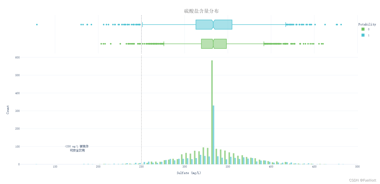
结论： 就硫酸盐水平而言，只有1.8%的水样是可以安全饮用的。

1.6导电率

    def pic_Conductivity():fig = px.histogram(data_full, x='Conductivity', color='Potability',template='plotly_white',marginal='box', opacity=0.7, nbins=100,color_discrete_sequence=[colors_green[3], colors_blue[3]],barmode='group', histfunc='count')fig.add_annotation(text='电导率在200~800的区间<br> 都是安全可饮用的',x=600, y=90, showarrow=False)fig.update_layout(font_family='monospace',title=dict(text='水体导电率分布图', x=0.5, y=0.95,font=dict(color=colors_dark[2], size=20)),xaxis_title_text='Conductivity (μS/cm)',yaxis_title_text='Count',legend=dict(x=1, y=0.96, bordercolor=colors_dark[4], borderwidth=0, tracegroupgap=5),bargap=0.3,)fig.show()return# pic_Conductivity()

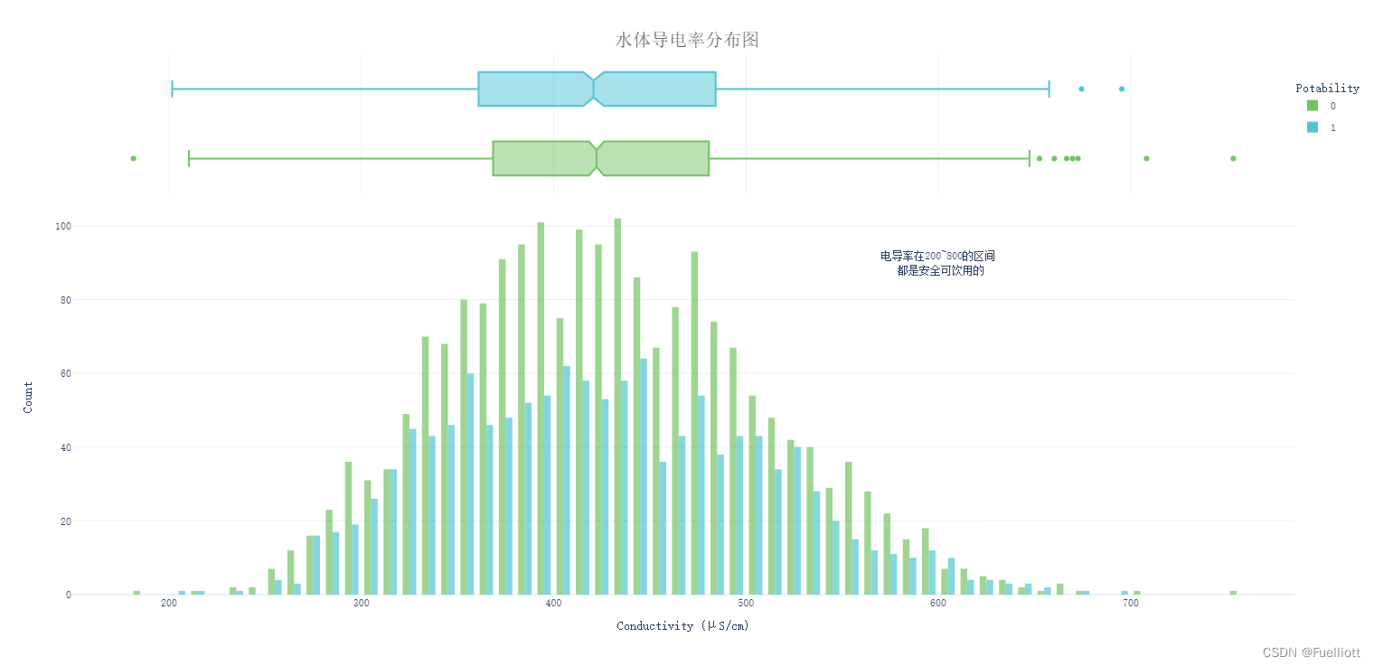
结论： 就导电率而言，近乎100%的数据集中的水样都是可以安全饮用的。

1.7有机碳

    def pic_Organic_carbon():fig = px.histogram(data_full, x='Organic_carbon', color='Potability',template='plotly_white',marginal='box', opacity=0.7, nbins=100,color_discrete_sequence=[colors_green[3], colors_blue[3]],barmode='group', histfunc='count')fig.add_vline(x=10, line_width=1, line_color=colors_dark[1], line_dash='dot', opacity=0.7)fig.add_annotation(text='一般有机碳的含量<br> 可高达 10 ppm', x=5.3, y=110, showarrow=False)fig.update_layout(font_family='monospace',title=dict(text='有机碳含量分布图', x=0.5, y=0.95,font=dict(color=colors_dark[2], size=20)),xaxis_title_text='Organic Carbon (ppm)',yaxis_title_text='Count',legend=dict(x=1, y=0.96, bordercolor=colors_dark[4], borderwidth=0, tracegroupgap=5),bargap=0.3,)fig.show()return# pic_Organic_carbon()

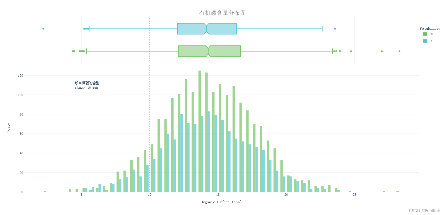
结论：数据集中90.6%的水质样本的碳含量高于饮用水中的常规碳含量（10 ppm）

1.8三卤甲烷

    def pic_Trihalomethanes():fig = px.histogram(data_full, x='Trihalomethanes', color='Potability',template='plotly_white',marginal='box', opacity=0.7, nbins=100,color_discrete_sequence=[colors_green[3], colors_blue[3]],barmode='group', histfunc='count')fig.add_vline(x=80, line_width=1, line_color=colors_dark[1], line_dash='dot', opacity=0.7)fig.add_annotation(text='三卤甲烷的含量上限<br> 是80 μg/L', x=115, y=90, showarrow=False)fig.update_layout(font_family='monospace',title=dict(text='三卤甲烷含量分布图', x=0.5, y=0.95,font=dict(color=colors_dark[2], size=20)),xaxis_title_text='Trihalomethanes (μg/L)',yaxis_title_text='Count',legend=dict(x=1, y=0.96, bordercolor=colors_dark[4], borderwidth=0, tracegroupgap=5),bargap=0.3,)fig.show()return# pic_Trihalomethanes()

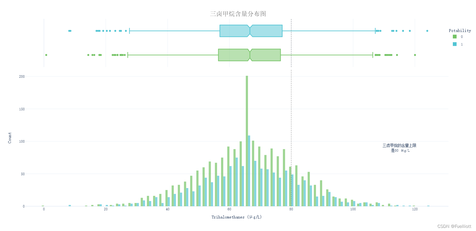
结论： 就水中三卤甲烷含量而言，76.6%的水样可安全饮用。

1.9浊度

    def pic_Turbidity():fig = px.histogram(data_full, x='Turbidity',  color='Potability', template='plotly_white',marginal='box', opacity=0.7, nbins=100,color_discrete_sequence=[colors_green[3], colors_blue[3]],barmode='group', histfunc='count')fig.add_vline(x=5, line_width=1, line_color=colors_dark[1], line_dash='dot', opacity=0.7)fig.add_annotation(text='<5 NTU 的浊度 <br> 被认为是安全的', x=6, y=90, showarrow=False)fig.update_layout(font_family='monospace',title=dict(text='水体浊度分布图', x=0.5, y=0.95,font=dict(color=colors_dark[2], size=20)),xaxis_title_text='Turbidity (NTU)',yaxis_title_text='Count',legend=dict(x=1, y=0.96, bordercolor=colors_dark[4], borderwidth=0, tracegroupgap=5),bargap=0.3,)fig.show()return# pic_Turbidity()

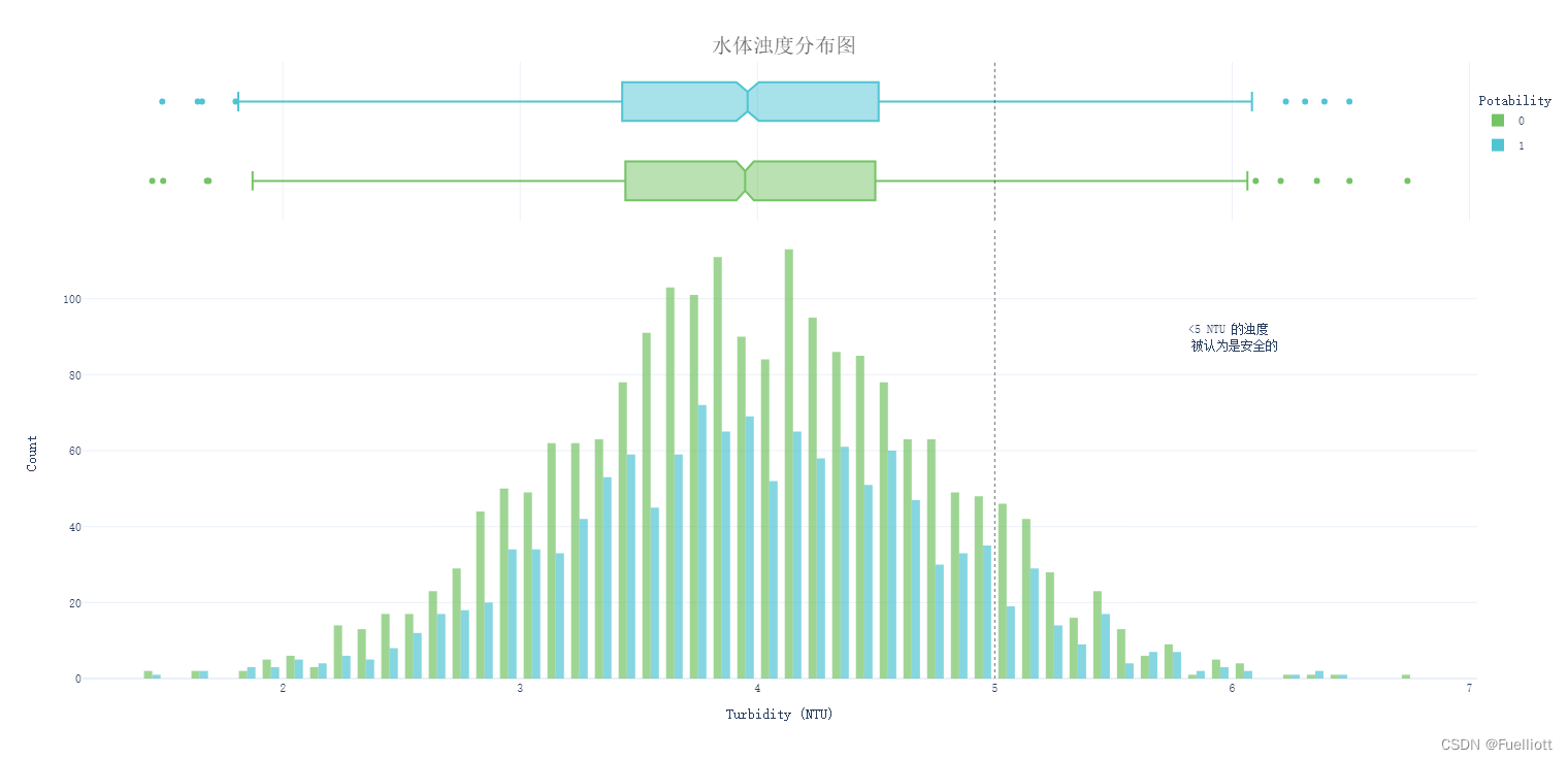
结论：就水样浊度而言，90.4%的水样可安全饮用。

2.水质的可饮用性数量统计

    def pic_1():# 设置画布plt.figure(figsize=(14, 6))plt.suptitle('水质的可饮用性数量统计', fontsize=20, weight='bold', fontproperties=zhfont1)plt.subplot(1, 2, 1)# 数量图sns.countplot(x=data_full['Potability'],  palette='husl')x=data_full['Potability'].value_counts().indexy=data_full['Potability'].value_counts().valuesfor a, b in zip(x, y):plt.text(a, 4*b/5, b, c='white',ha='center', va='bottom')# 扇形图数据names = ["Not Potable", "Potable"]values = data_full['Potability'].value_counts()colors = ["#E68193", "#459E97"]explode = (0.01, 0.01)# 作扇形图plt.subplot(1, 2, 2)plt.pie(x=values, labels=names, colors=colors, autopct='%1.0f%%', pctdistance=0.8, explode=explode)plt.show()print('数据集中有61%的不可饮用水数据和39%的可饮用水数据。')returnpic_1()

结论：数据集中存在39%的可饮用水与61%的不可饮用水。

3.可饮用水与非饮用水的各种特征分布比较

	 def pic_2():potable_0 = data_full.query("Potability == 0") #条件查询 输出dfpotable_1= data_full.query("Potability == 1")plt.figure(figsize=(10,8))plt.suptitle(' Distribution of features ', fontsize=20, weight='bold',color='#0A4361')for ax, col in enumerate(data_full.columns[:9]):plt.subplot(3, 3, ax + 1)plt.title(col)sns.kdeplot(x=potable_0[col], label="Non Potable", fill=True ,common_norm=False,color="#E68193", alpha=.8, linewidth=1)sns.kdeplot(x=potable_1[col], label="Potable", fill=True, common_norm=False, color="#459E97",alpha=.8, linewidth=1)plt.legend(loc='upper right',frameon=1,fontsize=6)plt.tight_layout()plt.show()

结论：可饮用水与非可饮用水之间，有机碳、PH值、浊度的数量分布差异不大。水体的硬度及硫酸盐含量比较影响该水体是否被划为可饮用水。

4.水质特征的相关性分析

    def pic_4():mask = np.zeros_like(data_full.corr(), dtype=np.bool_)mask[np.triu_indices_from(mask)] = Truefig, ax = plt.subplots(figsize=(13, 13))heatmap = sns.heatmap(data_full.corr(),mask=mask,square=True,linewidths=.5,cmap='PuBuGn',cbar_kws={'shrink': .4, "ticks": [-1, -.5, 0, 0.5, 1]},vmin=-1,vmax=1,annot=True,annot_kws={"size": 12})ax.set_yticklabels(data_full.corr(), rotation=0)ax.set_xticklabels(data_full.corr())sns.set_style({'xtick.bottom': True}, {'ytick.left': True})ax.set_title('水质特征的相关性', size=22, weight='bold', pad=20,fontproperties=zhfont1)plt.show()print('硫酸盐和固体含量存在相对的弱负相关影响。另外硫酸盐和硬度也有负相关趋势。')return

结论：各水质特征之间的相关系数很低，硫酸盐和固体含量存在相对的弱负相关影响。

三、水质可饮用性的预测

1.特征的预处理及选定合适的模型

	'把数据进行标准化'data_full = pd.read_csv(r'C:\xlwings\water\water_potability_full.csv', index_col=0)X = data_full.drop('Potability', axis=1).valuesy = data_full['Potability'].valuesX_train, X_test, y_train, y_test = train_test_split(X, y, test_size=0.3, random_state=101)scaler = StandardScaler()scaler.fit(X_train)X_train = scaler.transform(X_train)X_test = scaler.transform(X_test)'选择模型'filterwarnings('ignore')models = [("LR", LogisticRegression(max_iter=1000)), ("SVC", SVC()), ('KNN', KNeighborsClassifier(n_neighbors=10)),("DTC", DecisionTreeClassifier()), ("GNB", GaussianNB()),("SGDC", SGDClassifier()), ("Perc", Perceptron()), ("NC", NearestCentroid()),("Ridge", RidgeClassifier()), ("NuSVC", NuSVC()), ("BNB", BernoulliNB()),('RF', RandomForestClassifier()), ('ADA', AdaBoostClassifier()),('XGB', GradientBoostingClassifier()), ('PAC', PassiveAggressiveClassifier())]results = []names = []finalResults = []for name, model in models:model.fit(X_train, y_train)model_results = model.predict(X_test)score = precision_score(y_test, model_results, average='macro')results.append(score)names.append(name)finalResults.append((name, score))finalResults.sort(key=lambda k: k[1], reverse=True)k=len(finalResults)for i in range(k):print(finalResults[i]) 

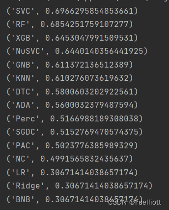
根据输出的准确度分数分析，选取SVC、RF、XGB这三个模型。

2.水质可饮用性的预测建模

 data_full = pd.read_csv(r'C:\xlwings\water\water_potability_full.csv', index_col=0)X = data_full.drop('Potability', axis=1).valuesy = data_full['Potability'].valuesmodel = VotingClassifier(estimators=[('XGB', GradientBoostingClassifier()),('RF', RandomForestClassifier()),('SVC', SVC())], voting='hard')accuracy = []scaler = StandardScaler()skf = RepeatedStratifiedKFold(n_splits=5, n_repeats=3)skf.get_n_splits(X, y)for train_index, test_index in skf.split(X, y):X_train, X_test = X[train_index], X[test_index]y_train, y_test = y[train_index], y[test_index]scaler.fit(X_train)X_train = scaler.transform(X_train)X_test = scaler.transform(X_test)model.fit(X_train, y_train)predictions = model.predict(X_test)score = accuracy_score(y_test, predictions)accuracy.append(score)print(np.mean(accuracy))

输出结果
0.6730798113324644

总结

1.数据集中92%的水质样本属于硬水性质。

2.数据种包含的酸性和碱性pH值水样数量几乎相等。

3.可饮用水的理想TDS最大限值为1000 mg/l，数据样本中绝大多数的TDS值都超标了20到40倍，存在数据单位差异的可能性，需要进一步探究。

4.就氯胺水平而言，只有2%的水样是可以安全饮用的。

5.就硫酸盐水平而言，只有1.8%的水样是可以安全饮用的。

6.就导电率而言，近乎100%的数据集中的水样都是可以安全饮用的。

7.数据集中90.6%的水质样本的碳含量高于饮用水中的常规碳含量（10 ppm）。

8.就水中三卤甲烷含量而言，76.6%的水样可安全饮用。

9.就水样浊度而言，90.4%的水样可安全饮用。

10.数据集中存在39%的可饮用水与61%的不可饮用水。

11.可饮用水与非可饮用水之间，有机碳、PH值、浊度的数量分布差异不大。水体的硬度及硫酸盐含量比较影响该水体是否被划为可饮用水。

12.各水质特征之间的相关系数很低，硫酸盐和固体含量存在相对的弱负相关影响。

13.Random Forest、XGBoost和SVC对模型的训练效果较好。

14.使用基于k折交叉验证的集成算法能得出准确度在67%左右。