Let There Be Color! Large-Scale Texturing of 3D Reconstructions 阅读笔记

Let There Be Color! Large-Scale Texturing of 3D Reconstructions

来到了三维重建的最后一部，纹理重建！

Abstract.

3D reconstruction pipelines using structure-from-motion and multi-view stereo techniques are today able to reconstruct impressive, large-scale geometry models from images but do not yield textured results(没有纹理，没有灵魂). Current texture creation methods are unable to handle the complexity and scale of these models. We therefore present the first comprehensive texturing framework for large-scale, real-world 3D reconstructions. Our method addresses most challenges occurring in such reconstructions: the large number of input images, their drastically varying properties such as image scale, (out-of-focus) blur, exposure variation, and occluders (e.g., moving plants or pedestrians). Using the proposed technique, we are able to texture datasets that are several orders of magnitude larger and far more challenging than shown in related work.

提出一个适用于以上情况的纹理建模方案

1 Introduction

In the last decade, 3D reconstruction from images has made tremendous progress. Camera calibration is now possible even on Internet photo collections [20] and for city scale datasets [1]. There is a wealth of dense multi-view stereo reconstruction algorithms, some also scaling to city level [7,8]. Realism is strongly increasing: Most recently Shan et al. [18] presented large reconstructions which are hard to distinguish from the input images if rendered at low resolution. Looking at the output of state of the art reconstruction algorithms one notices, however, that color information is still encoded as per-vertex color and therefore coupled to mesh resolution. （点的颜色仍然得到了保留）An important building block to make the reconstructed models a convincing experience for end users while keeping their size manageable is still missing: texture. Although textured models are common in the computer graphics context, texturing 3D reconstructions from images is very challenging due to illumination and exposure changes, non-rigid scene parts, unreconstructed occluding objects and image scales that may vary by several orders of magnitudes between close-up views and distant overview images.
So far, texture acquisition （纹理捕获）has not attracted nearly as much attention as geometry acquisition: Current benchmarks such as the Middlebury multi-view stereo benchmark [17] focus only on geometry and ignore appearance aspects. Furukawa et al. [8] produce and render point clouds with very limited resolution, which is especially apparent in close-ups. To texture the reconstructed geometry Frahm et al. [7] use the mean of all images that observe it which yields insufficient visual fidelity. Shan et al. [18] perform impressive work on estimating lighting parameters per input image and per-vertex reflectance parameters. Still, they use per-vertex colors and are therefore limited to the mesh resolution. Our texturing abilities seem to be lagging behind those of geometry reconstruction.

简言之，纹理重建远远落后集合重建

While there exists a significant body of work on texturing (Section 2 gives a detailed review) most authors focus on small, controlled datasets where the above challenges do not need to be taken into account. Prominent exceptions handle only specialized cases such as architectural scenes: Garcia-Dorado et al. [10] reconstruct and texture entire cities, but their method is specialized to the city setting as it uses a 2.5D scene representation (building outlines plus estimated elevation maps) and a sparse image set where each mesh face is visible in very few views. Also, they are restricted to regular block city structures with planar surfaces and treat buildings, ground, and building-ground transitions differently during texturing. Sinha et al. [19] texture large 3D models with planar surfaces (i.e., buildings) that have been created interactively using cues from structurefrom-motion on the input images. Since they only consider this planar case, they can optimize each surface independently. In addition, they rely on user interaction to mark occluding objects (e.g., trees) in order to ignore them during texturing. Similarly, Tan et al. [22] propose an interactive texture mapping approach for building fa¸cades. Stamos and Allen [21] operate on geometry data acquired with time-of-flight scanners and therefore need to solve a different set of problems including the integration of range and image data.
We argue that texture reconstruction is vitally important for creating realistic models without increasing their geometric complexity. It should ideally be fully automatic even for large-scale, real-world datasets. This is challenging due to the properties of the input images as well as unavoidable imperfections in the reconstructed geometry. Finally, a practical method should be efficient enough to handle even large models in a reasonable time frame. In this paper we therefore present the first unified texturing approach that handles large, realistic datasets reconstructed from images with a structure-from-motion plus multi-view stereo pipeline. Our method fully automatically accounts for typical challenges inherent in this setting and is efficient enough to texture real-world models with hundreds of input images and tens of millions of triangles within less than two hours.

emmm，看看就好

2 Related Work

Texturing a 3D model from multiple registered images is typically performed in a two step approach: First, one needs to select which view(s) should be used to texture each face yielding a preliminary texture. In the second step, this texture is optimized for consistency to avoid seams between adjacent texture patches.

1.选择要进行重建的view
2.进行连续化操作，避免空隙

View Selection The literature can be divided into two main classes: Several approaches select and blend multiple views per face to achieve a consistent texture across patch borders [5,13]. In contrast, many others texture each face with exactly one view [9,10,15,23]. Sinha et al. [19] also select one view, but per texel instead of per face. Some authors [2,6] propose hybrid approaches that generally select a single view per face but blend close to texture patch borders.
Blending images causes problems in a multi-view stereo setting: First, if camera parameters or the reconstructed geometry are slightly inaccurate, texture patches may be misaligned at their borders, produce ghosting, and result in strongly visible seams. This occurs also if the geometric model has a relatively low resolution and does not perfectly represent the true object geometry. Second, in realistic multi-view stereo datasets we often observe a strong difference in image scale: The same face may cover less than one pixel in one view and several thousand in another. If these views are blended, distant views blur out details from close-ups. This can be alleviated by weighting the images to be blended [5] or by blending in frequency space [2,6], but either way blending entails a quality loss because the images are resampled into a common coordinate frame.
Callieri et al. [5] compute weights for blending as a product of masks indicating the suitability of input image pixels for texturing with respect to angle, proximity to the model, and proximity to depth discontinuities. They do however not compute real textures but suggest the use of vertex colors in combination with mesh subdivision. This contradicts the purpose of textures (high resolution at low data cost) and is not feasible for large datasets or high-resolution images. Similarly, Grammatikopoulos et al. [13] blend pixels based on angle and proximity to the model. A view-dependent texturing approach that also blends views is Buehler et al.’s Lumigraph [4]. In contrast to the Lumigraph we construct a global textured model and abstain from blending.
Lempitsky and Ivanov [15] select a single view per face based on a pairwise Markov random field. Their data term judges the quality of views for texturing while their smoothness term models the severity of seams between texture patches. Based on this All`ene et al. [2] and Gal et al. [9] proposed data terms that incorporate additional effects compared to the basic data term. Since these methods form the base for our technique, we describe them in Section 3.
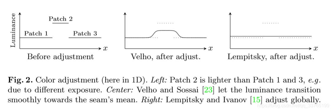
Color Adjustment After view selection the resulting texture patches may have strong color discontinuities due to exposure and illumination differences or even different camera response curves. Thus, adjacent texture patches need to be photometrically adjusted so that their seams become less noticeable. This can be done either locally or globally. Velho and Sossai [23] (Figure 2 (center)) adjust locally by setting the color at a seam to the mean of the left and right patch. They then use heat diffusion to achieve a smooth color transition towards this mean, which noticeably lightens Patches 1 and 3 at their borders. In contrast, Lempitsky and Ivanov [15] compute globally optimal luminance correction terms that are added to the vertex luminances subject to two intuitive constraints: After adjustment luminance differences at seams should be small and the derivative of adjustments within a texture patch should be small. This allows for a correction where Patch 2 is adjusted to the same level as Patch 1 and 3 (Figure 2 (right)) without visible meso- or large-scale luminance changes

看看前人的工作

3 Assumptions and Base Method

Our method takes as input a set of (typically several hundred) images of a scene that were registered using structure-from-motion [1,20]. Based on this the scene geometry is reconstructed using any current multi-view stereo technique (e.g., [7,8]) and further post-processed yielding a good (but not necessarily perfect) quality triangular mesh. （这里都是建立在前面的重建结果基础上的，并且这里要求表面重建的结果是三角网格）This setting ensures that the images are registered against the 3D reconstruction but also yields some inherent challenges: The structure-from-motion camera parameters may not be perfectly accurate and the reconstructed geometry may not represent the underlying scene perfectly. Furthermore, the input images may exhibit strong illumination, exposure, and scale differences and contain unreconstructed occluders such as pedestrians.
We now give an overview over how Lempitsky and Ivanov [15] and some related algorithms work since our approach is based on their work. Section 4 describes the key changes made in our approach to handle the above challenges.
The initial step in the pipeline is to determine the visibility of faces in the input images. Lempitsky and Ivanov then compute a labeling l that assigns a view l_i to be used as texture for each mesh face F_i using a pairwise Markov random field energy formulation (we use a simpler notation here):

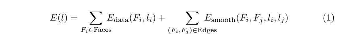
The data term E_data prefers “good” views for texturing a face. The smoothness term E_smooth minimizes seam (i.e., edges between faces textured with different images) visibility. E(l) is minimized with graph cuts and alpha expansion [3].
As data term the base method uses the angle between viewing direction and face normal. This is, however, insufficient for our datasets as it chooses images regardless of their proximity to the object, their resolution or their out-of-focus blur(失焦模糊). Allene et al. [2] project a face into a view and use the projection’s size as data term. This accounts for view proximity, angle and image resolution. Similar to this are the Lumigraph’s [4] view blending weights, which account for the very same effects. However, neither Allene nor the Lumigraph account for out-of-focus blur: In a close-up the faces closest to the camera have a large projection area and are preferred by All`ene’s data term or the Lumigraph weights but they may not be in focus and lead to a blurry texture. Thus, Gal et al. [9] use the gradient magnitude of the image integrated over the face’s projection. This term is large if the projection area is large (close, orthogonal images with a high resolution) or the gradient magnitude is large (in-focus images).
Gal et al. also introduce two additional degrees of freedom into the data term: They allow images to be translated by up to 64 pixels in x- or y-direction to minimize seam visibility. While this may improve the alignment of neighboring patches, we abstain from this because it only considers seam visibility and does not explain the input data. In a rendering of such a model a texture patch would have an offset compared to its source image. Also, these additional degrees of freedom may increase the computational complexity such that the optimization becomes infeasible for realistic dataset sizes. Lempitsky and Ivanov’s smoothness term is the difference between the texture to a seam’s left and right side integrated over the seam. This should prefer seams in regions where cameras are accurately registered or where misalignments are unnoticeable because the texture is smooth. We found, that computation of the seam error integrals is a computational bottleneck and cannot be precomputed due to the prohibitively large number of combinations. Furthermore, it favors distant or low-resolution views since a blurry texture produces smaller seam errors, an issue that does not occur in their datasets.
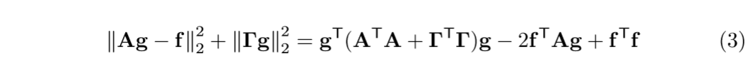
After obtaining a labeling from minimizing Equation 1, the patch colors are adjusted as follows: First, it must be ensured that each mesh vertex belongs to exactly one texture patch. Therefore each vertex on a seam is duplicated into two vertices: Vertex v_left belonging to the patch to the left and v_right belonging to the patch to the right of the seam.（ In the following, we only consider the case where seam vertices belong to n = 2 patches. For n>2 we create n copies of the vertex and optimize all pairs of those copies jointly, yielding a correction factor per vertex and patch.） Now each vertex v has a unique color f_v before adjustment. Then, an additive correction g_v is computed for each vertex, by minimizing the following expression (we use a simpler notation for clarity):

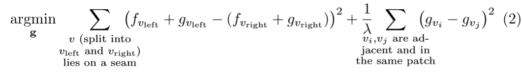
The first term ensures that the adjusted color to a seam’s left (f_vleft +g_vleft) and its right (f_vright + g_vright) are as similar as possible. The second term minimizes adjustment differences between adjacent vertices within the same texture patch. This favors adjustments that are as gradual as possible within a texture patch. After finding optimal g_v for all vertices the corrections for each texel are interpolated from the g_v of its surrounding vertices using barycentric coordinates. Finally, the corrections are added to the input images, the texture patches are packed into texture atlases, and texture coordinates are attached to the vertices.

上面这一大部分讲的是，首先是大体给每一个mash找到一个使用的贴纸，贴上（1），然后，再根据每一个vertex进行颜色上的的调整（2），最后就形成了一个完整的texture。
另外还介绍了好多前人的操作，有优点也有缺点，可大体了解下。
下面开始详细介绍了~

4 Large-Scale Texturing Approach

Following the base method we now explain our approach, focusing on the key novel aspects introduced to handle the challenges of realistic 3D reconstructions.

4.1 Preprocessing

We determine face visibility for all combinations of views and faces by first performing back face and view frustum culling（视域剔除）, before actually checking for occlusions. For the latter we employ a standard library [11] to compute intersections between the input model and viewing rays from the camera center to the triangle under question. This is more accurate than using rendering as, e.g., done by Callieri et al. [5], and has no relevant negative impact on performance. （直接使用一个标准库进行视域剔除 ）We then precompute the data terms for Equation 1 for all remaining face-view combinations since they are used multiple times during optimization, remain constant, and fit into memory (the table hasO(#faces·#views) entries and is very sparse).（预先计算公式1的数据项，并生成一个face - view的稀疏表）

4.2 View Selection

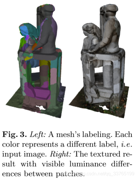
Our view selection follows the structure of the base algorithm, i.e., we obtain a labeling such as the one in Figure 3 (left) by optimizing Equation 1 with graph cuts and alpha expansion [3]. We, however, replace the base algorithm’s data and smoothness terms and augment the data term with a photo-consistency check.（改进）

Data Term For the reasons described in Section 3 we choose Gal et al.’s [9] data term

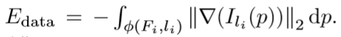
We compute the gradient magnitude ||∇(I_li)||₂ of the image into which face F_i is projected with a Sobel operator and sum over all pixels of the gradient magnitude image within F_i’s projection φ(F_i,l_i). If the projection contains less than one pixel we sample the gradient magnitude at the projection’s centroid and multiply it with the projection area.

在说E_data的计算方法，看的不是很明白。

The data term’s preference for large gradient magnitudes entails an important problem that Gal et al. do not account for because it does not occur in their controlled datasets: If a view contains an occluder such as a pedestrian that has not been reconstructed and can thus not be detected by the visibility check, this view should not be chosen for texturing the faces behind that occluder. （如果有遮挡，那么就不选择这个视图进行重建）Unfortunately this happens frequently with the gradient magnitude term (e.g. in Figure 9) because occluders such as pedestrians or leaves often feature a larger gradient magnitude than their background, e.g., a relatively uniform wall. We therefore introduce an additional step to ensure photo-consistency of the texture.

从以上来看，我们引入E_data的作用是为了选择能够用来重建的view，同时要消除遮挡物的影响。

Photo-Consistency Check We assume that for a specific face the majority of views see the correct color. A minority may see wrong colors (i.e., an occluder) and those are much less correlated. Based on this assumption Sinha et al. [19] and Grammatikopoulos et al. [13] use mean or median colors to reject inconsistent views. This is not sufficient, as we show in Section 5. Instead we use a slightly modified mean-shift algorithm consisting of the following steps:

1. Compute the face projection’s mean color c_i for each view i in which the face is visible. （在所有能看到face的view中计算此face的投影颜色均值）
2. Declare all views seeing the face as inliers. （将这些views标记为inliers）
3. Compute mean µ and covariance matrix Σ of all inliers’ mean color c_i.（计算所用inliers的颜色均值）
4. Evaluate a multi-variate Gaussian function
   
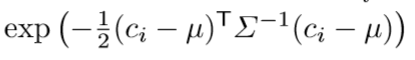
   for each view in which the face is visible. （计算每一个view的高斯值）
5. Clear the inlier list and insert all views whose function value is above a threshold (we use 6·10⁻³).
6. Repeat 3.–5. for 10 iterations or until all entries of Σ drop below 10⁻⁵, the inversion of Σ becomes unstable, or the number of inliers drops below 4.(结束条件)
   We obtain a list of photo-consistent views for each face and multiply a penalty on all other views’ data terms to prevent their selection. Note, that using the median instead of the mean does not work on very small query sets because for 3D vectors the marginal median is usually not a member of the query set so that too many views are purged. Not shifting the mean does not work in practice because the initial mean is often quite far away from the inliers’ mean (see Section 5 for an example). Sinha et al. [19] therefore additionally allow the user to interactively mark regions that should not be used for texturing, a step which we explicitly want to avoid.

通过上述的算法，选出每一个face的photo-consistent view list，能够很好地避免遮挡物的问题，另外，在计算时要用mean值而不是median值。

Smoothness Term As discussed above, Lempitsky and Ivanov’s smoothness term is a major performance bottleneck and counteracts our data term’s preference for close-up views. We propose a smoothness term based on the Potts model:

([·] is the Iverson bracket). This also prefers compact patches without favoring distant views and is extremely fast to compute.

简单粗暴，直接用iverson bracket决定E_smooth，解决了 Lempitsky and Ivanov’s smoothness term is a major performance bottleneck and counteracts our data term’s preference for close-up views. 的问题！而且效果还很好~

4.2的这一小节主要在讲如何解决选择view selection的问题，主要是围绕equation（1）展开，介绍E_data和E_smooth的计算问题。

4.3 Color Adjustment

Models obtained from the view selection phase (e.g., Figure 3 (right)) contain many color discontinuities between patches. These need to be adjusted to minimize seam visibility. We use an improved version of the base method’s global adjustment, followed by a local adjustment with Poisson editing [16].（这里要解决不连续的问题啦~）

Global Adjustment A serious problem with Lempitsky and Ivanov’s color adjustment is that f_vleft and f_vright in Equation 2 are only evaluated at a single location: the vertex v’s projection into the two images adjacent to the seam. If there are even small registration errors (which there always are), both projections do not correspond to exactly the same spot on the real object. Also, if both images have a different scale the looked up pixels span a different footprint in 3D. This may be irrelevant in controlled lab datasets, but in realistic multi-view stereo datasets the lookups from effectively different points or footprints mislead the global adjustment and produce artifacts.

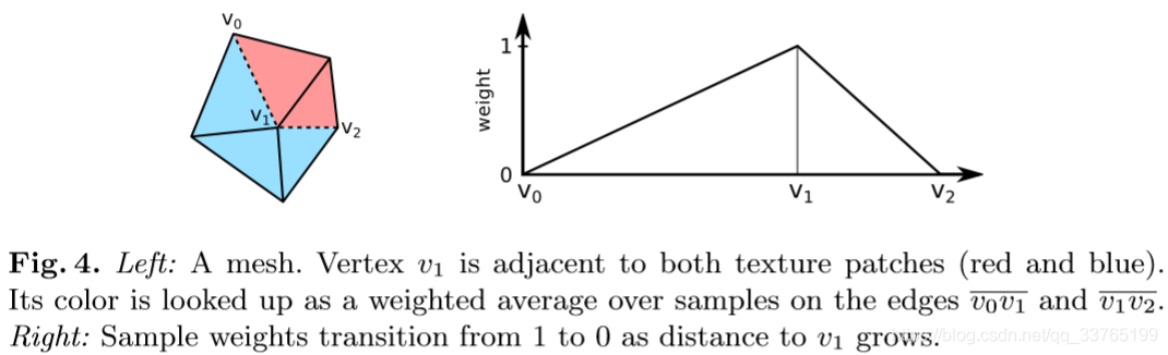
Color Lookup Support Region We alleviate this problem by not only looking up a vertex’ color value at the vertex projection but along all adjacent seam edges, as illustrated by Figure 4: Vertex v₁ is on the seam between the red and the blue patch. We evaluate its color in the red patch, f_v1,red, by averaging color samples from the red image along the two edges v₀v₁ and v₁v₂. On each edge we draw twice as many samples as the edge length in pixels. When averaging the samples we weight them according to Figure 4 (right): The sample weight is 1 on v₁ and decreases linearly with a sample’s distance to v₁. (The reasoning behind this is that after optimization of Equation 2 the computed correction g_v1,red is applied to the texels using barycentric coordinates. Along the seam the barycentric coordinates form the transition from 1 to 0.) We obtain average colors for the edges v₀v₁ and v₁v₂, which we average weighted with the edge lengths to obtain f_v1,red. Similarly we obtain f_v1,blue and insert both into Equation 2. For optimization, Equation 2 can now be written in matrix form as

这里贴上（2）的图进行比较：

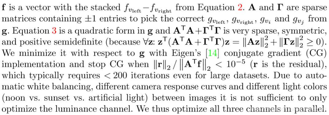
通过以上的变换，就能求出一个g，最重要的部分还是在Fig 4上_{说真的看不懂公式：）}

Poisson Editing Even with the above support regions Lempitsky and Ivanov’s global adjustment does not eliminate all visible seams, see an example in Figure 11 (bottom row, center). Thus, subsequent to global adjustment we additionally perform local Poisson image editing [16]. Gal et al. [9] do this as well, but in a way that makes the computation prohibitively expensive: They Poisson edit complete texture patches, which results in huge linear systems (with >107 variables for the largest patches in our datasets).*（出现了~ 泊松图像编辑~）
We thus restrict the Poisson editing of a patch to a 20 pixel wide border strip (shown in light blue in Figure 5). We use this strip’s outer rim (Fig. 5, dark blue) and inner rim (Fig. 5, red) as Poisson equation boundary conditions: We fix each outer rim pixel’s value to the mean of the pixel’s color in the image assigned to the patch and the image assigned to the neighboring patch. Each inner rim pixel’s value is fixed to its current color. If the patch is too small, we omit the inner rim. The Poisson equation’s guidance field is the strip’s Laplacian.

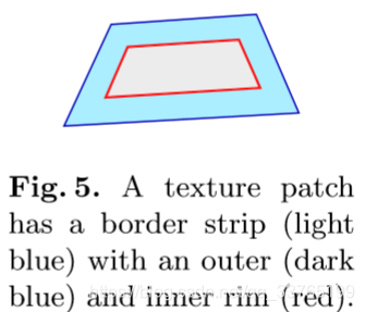
按照加粗的规则进行边缘值的分配

For all patches we solve the resulting linear systems in parallel with Eigen’s [14] SparseLU factorization. For each patch we only compute the factorization once and reuse it for all color channels because the system’s matrix stays the same. Adjusting only strips is considerably more time and memory efficient than adjusting whole patches. Note, that this local adjustment is a much weaker form of the case shown in Figure 2 (center) because patch colors have been adjusted globally beforehand. Also note, that we do not mix two images’ Laplacians and therefore still avoid blending.

说明性能优良，但是效果比不上global adjustment

后面的部分不是重点了，有兴趣就看看吧~

至此，texture reconstruction也结束了，总结起来也不是很复杂：首先选择view for faces，然后进行色彩生的调整与连续性调整。不过感觉里面还是有好多的有意思的思想没有挖掘出来，希望以后有机会再深入探讨吧~

最后，三维重建从图片的标定，到sfm，到mvs，再到表面重建和纹理重建就算全部完结了，也对三维重建的过程以及用得到的一些算法有了大致的了解~ 还是成就感爆棚~ 下一步可能会在SFM或者表面重建上继续发力~
祝大家国庆节快乐~
哈哈~