本文主要是介绍客户购买意愿预测,希望对大家解决编程问题提供一定的参考价值,需要的开发者们随着小编来一起学习吧!
目录
1.提出问题
2.理解数据
3.查看数据
4.数据分析
4.1离散变量分析
4.2连续变量分析
5.特征工程
5.1特征处理
5.2统计检验与特征筛选
5.3.不平衡数据集处理
6.数据建模
6.1构建模型以及模型评估
6.2方案实施
1.提出问题
本项目是与葡萄牙银行机构的营销活动相关。这些营销活动一般以电话为基础,银行的客服人员至少联系客户一次,以确认客户是否有意愿购买该银行的产品(定期存款)。
因此本文的任务是基本类型为分类任务,即预测客户是否购买该银行的产品。
2.理解数据
数据来源:https://www.kesci.com/home/competition/5c234c6626ba91002bfdfdd3/content/1
项目提供了2个数据集,分别为训练数据(train_set)、测试数据(test_set)
了解数据字段:
| NO | 字段名称 | 数据类型 | 字段描述 | |
|---|---|---|---|---|
| 1 | ID | Int | 客户唯一标识 | |
| 2 | age | Int | 客户年龄 | |
| 3 | job | String | 客户的职业 | |
| 4 | marital | String | 婚姻状况 | |
| 5 | education | String | 受教育水平 | |
| 6 | default | String | 是否有违约记录 | |
| 7 | balance | Int | 每年账户的平均余额 | |
| 8 | housing | String | 是否有住房贷款 | |
| 9 | loan | String | 是否有个人贷款 | |
| 10 | contact | String | 与客户联系的沟通方式 | |
| 11 | day | Int | 最后一次联系的时间(几号) | |
| 12 | month | String | 最后一次联系的时间(月份) | |
| 13 | duration | Int | 最后一次联系的交流时长 | |
| 14 | campaign | Int | 在本次活动中,与该客户交流过的次数 | |
| 15 | pdays | Int | 距离上次活动最后一次联系该客户,过去了多久(999表示没有联系过) | |
| 16 | previous | Int | 在本次活动之前,与该客户交流过的次数 | |
| 17 | poutcome | String | 上一次活动的结果 | |
| 18 | y | Int | 预测客户是否会订购定期存款业务 |
3.查看数据
In [1]:
import pandas as pd
import numpy as np
import matplotlib.pyplot as plt
import seaborn as snsplt.rcParams['font.sans-serif'] = ['SimHei']
plt.rcParams['axes.unicode_minus'] = Falseimport  warnings
warnings.filterwarnings("ignore")
In [2]:
train=pd.read_csv('D:/data/predict/train_set.csv')
test=pd.read_csv('D:/data/predict/test_set.csv')
train.head()
Out[2]:
| ID | age | job | marital | education | default | balance | housing | loan | contact | day | month | duration | campaign | pdays | previous | poutcome | y | |
|---|---|---|---|---|---|---|---|---|---|---|---|---|---|---|---|---|---|---|
| 0 | 1 | 43 | management | married | tertiary | no | 291 | yes | no | unknown | 9 | may | 150 | 2 | -1 | 0 | unknown | 0 |
| 1 | 2 | 42 | technician | divorced | primary | no | 5076 | yes | no | cellular | 7 | apr | 99 | 1 | 251 | 2 | other | 0 |
| 2 | 3 | 47 | admin. | married | secondary | no | 104 | yes | yes | cellular | 14 | jul | 77 | 2 | -1 | 0 | unknown | 0 |
| 3 | 4 | 28 | management | single | secondary | no | -994 | yes | yes | cellular | 18 | jul | 174 | 2 | -1 | 0 | unknown | 0 |
| 4 | 5 | 42 | technician | divorced | secondary | no | 2974 | yes | no | unknown | 21 | may | 187 | 5 | -1 | 0 | unknown | 0 |
In [3]:
print('训练数据集大小', train.shape,'测试数据集大小',test.shape)
训练数据集大小 (25317, 18) 测试数据集大小 (10852, 17)
In [4]:
# 从训练集查看是否平衡数据集
plt.rc('font', family='SimHei', size=13)
fig = plt.figure()
plt.pie(train['y'].value_counts(),labels=train['y'].value_counts().index,autopct='%1.2f%%',counterclock = False)
plt.title('购买率')
plt.show()
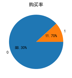
数据集是不平衡数据集
In [5]:
# 查看是否有空值
data = pd.concat([train.drop(['y'],axis=1),test],axis=0).reset_index(drop=True)
data.isnull().sum()
无空值
In [7]:
# 对object型数据查看unique
str_features = []
num_features=[]
for col in train.columns:if train[col].dtype=='object':str_features.append(col)print(col,':  ',train[col].unique())if train[col].dtype=='int64' and col not in ['ID','y']:num_features.append(col)
job :   ['management' 'technician' 'admin.' 'services' 'retired' 'student''blue-collar' 'unknown' 'entrepreneur' 'housemaid' 'self-employed''unemployed']
marital :   ['married' 'divorced' 'single']
education :   ['tertiary' 'primary' 'secondary' 'unknown']
default :   ['no' 'yes']
housing :   ['yes' 'no']
loan :   ['no' 'yes']
contact :   ['unknown' 'cellular' 'telephone']
month :   ['may' 'apr' 'jul' 'jun' 'nov' 'aug' 'jan' 'feb' 'dec' 'oct' 'sep' 'mar']
poutcome :   ['unknown' 'other' 'failure' 'success']
观察发现分类字段有‘unknown’这个类别,此时将该类别也当作缺失值,进一步查看
In [8]:
train.isin(['unknown']).mean()*100
Out[8]:
ID            0.000000
age           0.000000
job           0.643836
marital       0.000000
education     4.206660
default       0.000000
balance       0.000000
housing       0.000000
loan          0.000000
contact      28.759332
day           0.000000
month         0.000000
duration      0.000000
campaign      0.000000
pdays         0.000000
previous      0.000000
poutcome     81.672394
y             0.000000
dtype: float64
通常对于缺失值的处理,最常用的方法无外乎删除法、替换法和插补法。
- 删除法是指将缺失值所在的观测行删除(前提是缺失行的比例非常低,如5%以内),或者删除缺失值所对应的变量(前提是该变量中包含的缺失值比例非常高,如70%左右)
- 替换法是指直接利用缺失变量的均值、中位数或众数替换该变量中的缺失值,其好处是缺失值的处理速度快,弊端是易产生有偏估计,导致缺失值替换的准确性下降
- 插补法则是利用有监督的机器学习方法(如回归模型、树模型、网络模型等)对缺失值作预测,其优势在于预测的准确性高,缺点是需要大量的计算,导致缺失值的处理速度大打折扣
这里观察到contact和poutcome的‘unknow’类别分别达到28.76%和81.67%,在展示数据后考虑进一步处理,job和education的unknown占比较小,考虑不对这两个特征的unknow进行处理
In [9]:
print(str_features)
print(num_features)
['job', 'marital', 'education', 'default', 'housing', 'loan', 'contact', 'month', 'poutcome']
['age', 'balance', 'day', 'duration', 'campaign', 'pdays', 'previous']
4.数据分析
4.1离散变量分析
In [10]:
plt.figure(figsize=(15,15))
i=1
for col in str_features:plt.subplot(3,3,i)# 这里用mean是因为标签是0,1二分类,0*0的行数(即没购买的人数)+1*1的行数(购买的人数)/所有行数=购买率train.groupby([col])['y'].mean().plot(kind='bar',stacked=True,rot=90,title='Purchase rate of {}'.format(col))plt.subplots_adjust(wspace=0.2,hspace=0.7)  # 调整子图间距i=i+1
plt.show()

结论:通过可视图可以初步观察到这些特征是否会影响购买率
4.2连续变量分析
In [11]:
num_features
Out[11]:
['age', 'balance', 'day', 'duration', 'campaign', 'pdays', 'previous']In [12]:
train[num_features].describe()
Out[12]:
| age | balance | day | duration | campaign | pdays | previous | |
|---|---|---|---|---|---|---|---|
| count | 25317.000000 | 25317.000000 | 25317.000000 | 25317.000000 | 25317.000000 | 25317.000000 | 25317.000000 |
| mean | 40.935379 | 1357.555082 | 15.835289 | 257.732393 | 2.772050 | 40.248766 | 0.591737 |
| std | 10.634289 | 2999.822811 | 8.319480 | 256.975151 | 3.136097 | 100.213541 | 2.568313 |
| min | 18.000000 | -8019.000000 | 1.000000 | 0.000000 | 1.000000 | -1.000000 | 0.000000 |
| 25% | 33.000000 | 73.000000 | 8.000000 | 103.000000 | 1.000000 | -1.000000 | 0.000000 |
| 50% | 39.000000 | 448.000000 | 16.000000 | 181.000000 | 2.000000 | -1.000000 | 0.000000 |
| 75% | 48.000000 | 1435.000000 | 21.000000 | 317.000000 | 3.000000 | -1.000000 | 0.000000 |
| max | 95.000000 | 102127.000000 | 31.000000 | 3881.000000 | 55.000000 | 854.000000 | 275.000000 |
#用热力图考察数值型特征与目标之间的关系
num_train = train[['age', 'balance', 'day', 'duration', 'campaign', 'pdays', 'previous','y']]
plt.figure(figsize = (10,8))
corr = num_train.corr()
sns.heatmap(corr ,annot=True, cmap= 'Spectral_r')
<matplotlib.axes._subplots.AxesSubplot at 0x23a886ed9a0>
从中可见duration(最后一次联系的交流时长)和是否购买之间存在着较大的相关性, balance存在着较低的相关性, 特征previous和pdays, campaign和day之间相关性较强。
age 年龄
In [13]:
plt.figure()
sns.boxenplot(x='y', y=u'age', data=train)
plt.show()

In [14]:
train[train['y']==0]['age'].plot(kind='kde',label='0')
train[train['y']==1]['age'].plot(kind='kde',label='1')
plt.legend()
plt.show()

两类客户的购买年龄分布差异不大;
balance 每年账户的平均余额
In [15]:
train['balance'].plot(kind='hist')
plt.show()
duration 最后一次联系的交流时长
In [16]:
plt.figure()
sns.boxplot(y=u'duration', data=train)
plt.show()

campaign 在本次活动中,与该客户交流过的次数
In [17]:
plt.figure(figsize=(10,5))
plt.subplot(1,2,1)
sns.boxenplot(x='y', y=u'campaign', data=train)
plt.subplot(1,2,2)
sns.boxplot(y=u'campaign', data=train)
plt.show()

pdays 距离上次活动最后一次联系该客户,过去了多久(999表示没有联系过)
In [18]:
plt.figure(figsize=(10,5))
plt.subplot(1,2,1)
sns.boxenplot(x='y', y=u'pdays', data=train)
plt.subplot(1,2,2)
sns.boxplot(y=u'pdays', data=train)
plt.show()

previous 在本次活动之前,与该客户交流过的次数
In [19]:
plt.figure(figsize=(10,5))
plt.subplot(1,2,1)
sns.boxenplot(x='y', y=u'previous', data=train)
plt.subplot(1,2,2)
sns.boxplot(y=u'previous', data=train)
plt.show()
5.特征工程
In [20]:
from scipy.stats import chi2_contingency       # 数值型特征检验,检验特征与标签的关系
from scipy.stats import f_oneway,ttest_ind     # 分类型特征检验,检验特征与标签的关系
In [21]:
#----------数据集处理--------------#
from sklearn.model_selection import train_test_split        # 划分训练集和验证集
from sklearn.model_selection import KFold,StratifiedKFold   # k折交叉
from imblearn.combine import SMOTETomek,SMOTEENN            # 综合采样
from imblearn.over_sampling import SMOTE                    # 过采样
from imblearn.under_sampling import RandomUnderSampler      # 欠采样#----------数据处理--------------#
from sklearn.preprocessing import StandardScaler # 标准化
from sklearn.preprocessing import OneHotEncoder  # 热独编码
from sklearn.preprocessing import OrdinalEncoder
5.1特征处理
数据清洗的步骤为:选择子集——列名重命名——删除重复值——缺失值处理——数据类型转换——数据排序——异常值处理,在这个案例中,在查看空值与缺失值以及对数据的可视化观测后,对连续变量检测异常值后进行处理,保留所有离散变量,并对其做虚拟变量处理。
连续变量即数值化数据做异常值处理
In [22]:
# 异常值处理
def outlier_processing(dfx):df = dfx.copy()q1 = df.quantile(q=0.25)q3 = df.quantile(q=0.75)iqr = q3 - q1Umin = q1 - 1.5*iqrUmax = q3 + 1.5*iqr df[df>Umax] = df[df<=Umax].max()df[df<Umin] = df[df>=Umin].min()return df
In [23]:
train['age']=outlier_processing(train['age'])
train['day']=outlier_processing(train['day'])
train['duration']=outlier_processing(train['duration'])
train['campaign']=outlier_processing(train['campaign'])test['age']=outlier_processing(test['age'])
test['day']=outlier_processing(test['day'])
test['duration']=outlier_processing(test['duration'])
test['campaign']=outlier_processing(test['campaign'])
In [24]:
train[num_features].describe()
Out[24]:
| age | balance | day | duration | campaign | pdays | previous | |
|---|---|---|---|---|---|---|---|
| count | 25317.000000 | 25317.000000 | 25317.000000 | 25317.000000 | 25317.000000 | 25317.000000 | 25317.000000 |
| mean | 40.859502 | 1357.555082 | 15.835289 | 234.235138 | 2.391437 | 40.248766 | 0.591737 |
| std | 10.387365 | 2999.822811 | 8.319480 | 175.395559 | 1.599851 | 100.213541 | 2.568313 |
| min | 18.000000 | -8019.000000 | 1.000000 | 0.000000 | 1.000000 | -1.000000 | 0.000000 |
| 25% | 33.000000 | 73.000000 | 8.000000 | 103.000000 | 1.000000 | -1.000000 | 0.000000 |
| 50% | 39.000000 | 448.000000 | 16.000000 | 181.000000 | 2.000000 | -1.000000 | 0.000000 |
| 75% | 48.000000 | 1435.000000 | 21.000000 | 317.000000 | 3.000000 | -1.000000 | 0.000000 |
| max | 70.000000 | 102127.000000 | 31.000000 | 638.000000 | 6.000000 | 854.000000 | 275.000000 |
分类变量做编码处理
In [25]:
dummy_train=train.join(pd.get_dummies(train[str_features])).drop(str_features,axis=1).drop(['ID','y'],axis=1)
dummy_test=test.join(pd.get_dummies(test[str_features])).drop(str_features,axis=1).drop(['ID'],axis=1)
5.2统计检验与特征筛选
连续变量-连续变量 相关分析
连续变量-分类变量 T检验/方差分析
分类变量-分类变量 卡方检验
对类别标签(离散变量)用卡方检验分析重要性
卡方检验认为显著水平大于95%是差异性显著的,这里即看p值是否是p>0.05,若p>0.05,则说明特征不会呈现差异性。
In [26]:
for col in str_features:obs=pd.crosstab(train['y'],train[col],rownames=['y'],colnames=[col])chi2, p, dof, expect = chi2_contingency(obs)print("{} 卡方检验p值: {:.4f}".format(col,p))
job 卡方检验p值: 0.0000
marital 卡方检验p值: 0.0000
education 卡方检验p值: 0.0000
default 卡方检验p值: 0.0001
housing 卡方检验p值: 0.0000
loan 卡方检验p值: 0.0000
contact 卡方检验p值: 0.0000
month 卡方检验p值: 0.0000
poutcome 卡方检验p值: 0.0000
结果显示所有类型变量均显著。
对连续变量做方差分析进行特征筛选
In [27]:
from sklearn.feature_selection import SelectKBest,f_classiff,p=f_classif(train[num_features],train['y'])
k = f.shape[0] - (p > 0.05).sum()
selector = SelectKBest(f_classif, k=k)
selector.fit(train[num_features],train['y'])print('scores_:',selector.scores_)
print('pvalues_:',selector.pvalues_)
print('selected index:',selector.get_support(True))
scores_: [  13.38856992   84.16396612   25.76507245 4405.56959938  193.97418155296.33099313  199.09942912]
pvalues_: [2.53676251e-04 4.89124305e-20 3.88332900e-07 0.00000000e+006.26768275e-44 4.93591331e-66 4.86613654e-45]
selected index: [0 1 2 3 4 5 6]
结果显示所有连续变量均显著。
In [28]:
# 标准化,返回值为标准化后的数据
standardScaler=StandardScaler()
ss=standardScaler.fit(dummy_train.loc[:,num_features])
dummy_train.loc[:,num_features]=ss.transform(dummy_train.loc[:,num_features])
dummy_test.loc[:,num_features]=ss.transform(dummy_test.loc[:,num_features])
5.3.不平衡数据集处理
In [29]:
X=dummy_train
y=train['y']
先拆分数据集为训练集和验证集,对训练集做采样处理,验证集不动
In [30]:
X_train,X_valid,y_train,y_valid=train_test_split(X,y,test_size=0.2,random_state=2021)
In [31]:
smote_tomek = SMOTETomek(random_state=2021)
X_resampled, y_resampled = smote_tomek.fit_resample(X_train, y_train)
6.数据建模
6.1构建模型以及模型评估
In [41]:
#----------建模工具--------------#
from sklearn.model_selection import GridSearchCV
from sklearn.pipeline import Pipelineimport lightgbm as lgb
from sklearn.linear_model import LogisticRegression
from sklearn.tree import DecisionTreeClassifier
from sklearn.ensemble import RandomForestClassifier
from sklearn.svm import SVC
from sklearn.neighbors import KNeighborsClassifier
In [42]:
#----------模型评估工具----------#
from sklearn.metrics import confusion_matrix # 混淆矩阵
from sklearn.metrics import classification_report
from sklearn.metrics import recall_score,f1_score
from sklearn.metrics import roc_auc_score
from sklearn.metrics import roc_curve
本文主要考虑逻辑回归、支持向量机、随机森林和LGBM算法
In [43]:
#逻辑回归
param = {"penalty": ["l1", "l2", ], "C": [0.1, 1, 10], "solver": ["liblinear","saga"]}
gs = GridSearchCV(estimator=LogisticRegression(), param_grid=param, cv=2, scoring="roc_auc",verbose=10)
gs.fit(X_resampled,y_resampled)
print(gs.best_params_)
y_pred = gs.best_estimator_.predict(X_valid)
print(classification_report(y_valid, y_pred))
{'C': 1, 'penalty': 'l2', 'solver': 'liblinear'}precision    recall  f1-score   support0       0.93      0.94      0.93      44681       0.51      0.51      0.51       596accuracy                           0.88      5064macro avg       0.72      0.72      0.72      5064
weighted avg       0.88      0.88      0.88      5064
In [44]:
# 训练集
confusion_matrix(y_resampled,gs.best_estimator_.predict(X_resampled),labels=[1,0])
Out[44]:
array([[16129, 1742],[ 1080, 16791]], dtype=int64)In [45]:
# 验证集
confusion_matrix(y_valid,y_pred,labels=[1,0])
Out[45]:
array([[ 302, 294],[ 290, 4178]], dtype=int64)In [46]:
#画roc-auc曲线
def get_rocauc(X,y,clf):from sklearn.metrics import roc_curveFPR,recall,thresholds=roc_curve(y,clf.predict_proba(X)[:,1],pos_label=1)area=roc_auc_score(y,clf.predict_proba(X)[:,1])maxindex=(recall-FPR).tolist().index(max(recall-FPR))threshold=thresholds[maxindex]plt.figure()plt.plot(FPR,recall,color='red',label='ROC curve (area = %0.2f)'%area)plt.plot([0,1],[0,1],color='black',linestyle='--')plt.scatter(FPR[maxindex],recall[maxindex],c='black',s=30)plt.xlim([-0.05,1.05])plt.ylim([-0.05,1.05])plt.xlabel('False Positive Rate')plt.ylabel('Recall')plt.title('Receiver operating characteristic example')plt.legend(loc='lower right')plt.show()return threshold
In [47]:
threshold=get_rocauc(X_resampled, y_resampled,gs.best_estimator_)

左上角的点即是Recall和FPR平衡的点,threshold即为平衡点对应的阀值。 可以根据阀值重新来构建预测结果:
In [48]:
# 阈值调整
def get_ypred(X,clf,threshold):y_pred=[]for i in clf.predict_proba(X)[:,1]:if i > threshold:y_pred.append(1)else:y_pred.append(0)return y_pred# ytrain_pred=get_ypred(Xtrain,clf,threshold)
In [49]:
# 支持向量机
param = {"C": list(np.linspace(0,1,10))}
gs = GridSearchCV(estimator=SVC(probability=True), param_grid=param, cv=2, scoring="roc_auc", n_jobs=-1, verbose=10)
gs.fit(X_resampled,y_resampled)
print(gs.best_params_)
y_pred = gs.best_estimator_.predict(X_valid)
print(classification_report(y_valid, y_pred))
Fitting 2 folds for each of 10 candidates, totalling 20 fits
{'C': 1.0}precision    recall  f1-score   support0       0.94      0.93      0.94      44681       0.52      0.58      0.55       596accuracy                           0.89      5064macro avg       0.73      0.75      0.74      5064
weighted avg       0.89      0.89      0.89      5064
In [53]:
# 随机森林
param = {'n_estimators':[500,520,530],'max_features':[0.74,0.75,0.77],'min_samples_leaf':[2,3,4]}
gs = GridSearchCV(estimator=RandomForestClassifier(), param_grid=param, cv=2, scoring="roc_auc", n_jobs=-1, verbose=10)
gs.fit(X_resampled,y_resampled)
print(gs.best_params_)
y_pred = gs.best_estimator_.predict(X_valid)
print(classification_report(y_valid, y_pred))
Fitting 2 folds for each of 27 candidates, totalling 54 fits
{'max_features': 0.74, 'min_samples_leaf': 2, 'n_estimators': 530}precision    recall  f1-score   support0       0.95      0.92      0.93      44681       0.51      0.64      0.57       596accuracy                           0.89      5064macro avg       0.73      0.78      0.75      5064
weighted avg       0.90      0.89      0.89      5064
In [56]:
from lightgbm.sklearn import LGBMClassifier
param = {'max_depth': [5,7,9,11,13],'learning_rate': [0.01,0.03,0.05,0.1],'num_leaves': [30,90,120],'n_estimators': [1000,1500,2000,2500]}
gs = GridSearchCV(estimator=LGBMClassifier(), param_grid=param, cv=5, scoring="roc_auc", n_jobs=-1, verbose=10)
gs.fit(X_resampled,y_resampled)
print(gs.best_params_)
y_pred = gs.best_estimator_.predict(X_valid)
print(classification_report(y_valid, y_pred))
Fitting 5 folds for each of 240 candidates, totalling 1200 fits
{'learning_rate': 0.01, 'max_depth': 13, 'n_estimators': 2000, 'num_leaves': 120}precision    recall  f1-score   support0       0.94      0.95      0.94      44681       0.59      0.53      0.56       596accuracy                           0.90      5064macro avg       0.77      0.74      0.75      5064
weighted avg       0.90      0.90      0.90      5064
from sklearn.metrics import roc_auc_score
LR_auc = roc_auc_score(y_valid, gs1.best_estimator_.predict_proba(X_valid)[:, 1])
svc_auc = roc_auc_score(y_valid, gs2.best_estimator_.predict_proba(X_valid)[:, 1])
rf_auc = roc_auc_score(y_valid, gs3.best_estimator_.predict_proba(X_valid)[:, 1])
LGBM_auc = roc_auc_score(y_valid, gs4.best_estimator_.predict_proba(X_valid)[:, 1])print("AUC for LR: {:.3f}".format(LR_auc))
print("AUC for SVC: {:.3f}".format(svc_auc))
print("AUC for Random Forest: {:.3f}".format(rf_auc))
print("AUC for LGBM: {:.3f}".format(LGBM_auc))
AUC for LR: 0.894
AUC for SVC: 0.907
AUC for Random Forest: 0.917
AUC for LGBM: 0.9266.2方案实施
通过对比逻辑回归、支持向量机、随机森林和LGBM算法的AUC得出最佳参数所构建的模型,得出LGBM算法参数为{'learning_rate': 0.01, 'max_depth': 13, 'n_estimators': 2000, 'num_leaves': 120}时效果最好,precision、recall、f1-score的weighted avg都为0.9,AUC最高为0.926。
In [57]:
X_test = dummy_test
y_test=gs.best_estimator_.predict_proba(X_test)
test['pred']=y_test[:,1]
In [58]:
test[['ID','pred']].to_csv('lgb.csv')
提交结果,最终得分:0.9253091
这篇关于客户购买意愿预测的文章就介绍到这儿,希望我们推荐的文章对编程师们有所帮助!