本文主要是介绍因子分析的一个小例子,希望对大家解决编程问题提供一定的参考价值,需要的开发者们随着小编来一起学习吧!
这是学习笔记的第 1997 篇文章
今天做了下因子分析中的东东,本来想找一些公共网站的数据,限于时间和要做一些数据整理,时间来不及,就找了一个现成的数据源。
这是洛杉矶等十二个大都市的人口调查获得的,包含了5个社会以经济变量:人口总数,居民受教育年限,佣人总数,服务行业人数,中等的房价。
为了方便我把数据集先提供出来。
| 人口(X1) | 教育年限(X2) | 佣人数(X3) | 服务人数(X4) | 房价(X5) |
| 5700 | 12.8 | 2500 | 270 | 25000 |
| 1000 | 10.9 | 600 | 10 | 10000 |
| 3400 | 8.8 | 1000 | 10 | 9000 |
| 3800 | 13.6 | 1700 | 140 | 25000 |
| 4000 | 12.8 | 1600 | 140 | 25000 |
| 8200 | 8.3 | 2600 | 60 | 12000 |
| 1200 | 11.4 | 400 | 10 | 16000 |
| 9100 | 11.5 | 3300 | 60 | 14000 |
| 9900 | 12.5 | 3400 | 180 | 18000 |
| 9600 | 13.7 | 3600 | 390 | 25000 |
| 9600 | 9.6 | 3300 | 80 | 12000 |
| 9400 | 11.4 | 4000 | 100 | 13000 |
我们把数据存储在excel里面,然后使用R语言来做分析。
首先导入数据,如果程序包openxlsx没有的话,就在R语言里安装下依赖。假设文件的路径是 D:\\yinzifenxi.xlsx
library(openxlsx)
读取excel的数据
data1 <- read.xlsx("D:\\yinzifenxi.xlsx" )
输出部分信息
> head(data1)
人口(X1) 教育(X2) 佣人(X3) 服务(X4) 房价(X5)
1 5700 12.8 2500 270 25000
2 1000 10.9 600 10 10000
3 3400 8.8 1000 10 9000
4 3800 13.6 1700 140 25000
5 4000 12.8 1600 140 25000
6 8200 8.3 2600 60 12000
>
> data1_cor <- cor(data1)
> head(cor(data1),5)
> head(cor(data1),5)
人口(X1) 教育(X2) 佣人(X3) 服务(X4) 房价(X5)
人口(X1) 1.00000000 0.00975059 0.9724483 0.4388708 0.02241157
教育(X2) 0.00975059 1.00000000 0.1542838 0.6914082 0.86307009
佣人(X3) 0.97244826 0.15428378 1.0000000 0.5147184 0.12192599
服务(X4) 0.43887083 0.69140824 0.5147184 1.0000000 0.77765425
房价(X5) 0.02241157 0.86307009 0.1219260 0.7776543 1.00000000
>
> library(psych)
确定因子数量
> fa.parallel(data1_cor, n.obs = 112, fa = "both", n.iter = 100)
Parallel analysis suggests that the number of factors = 2 and the number of components = 2
There were 18 warnings (use warnings() to see them)
得到的碎石图如下:
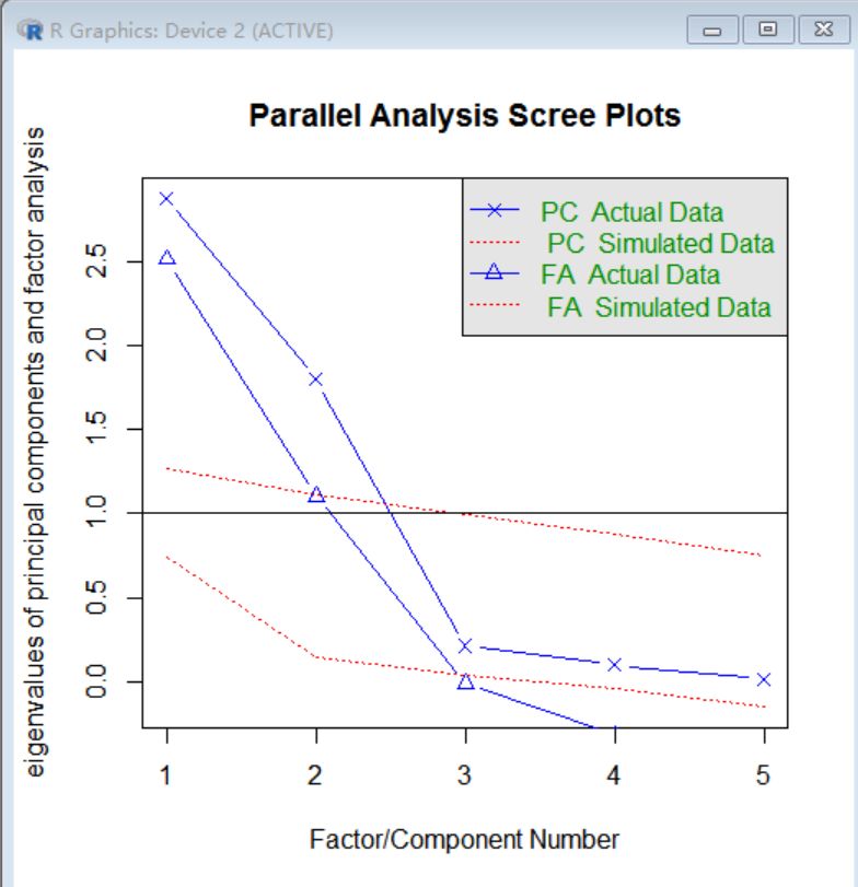
从这样的数据分析可以看到前2个会占据主要的部分,保留2个主成分即可。
接下来要做因子分析了,第一个参数是数据,第二个参数说明要保留两个主成分,第三个参数为旋转方法,为none,先不进行主成分旋转,第四个参数表示提取公因子的方法为最大似然法,不是机器学习的意思。
> fa_model1 <- fa(data1_cor, nfactors = 2, rotate = "none", fm = "ml")
输出分析的结果内容:
> fa_model1
Factor Analysis using method = ml
Call: fa(r = data1_cor, nfactors = 2, rotate = "none", fm = "ml")
Standardized loadings (pattern matrix) based upon correlation matrix
ML2 ML1 h2 u2 com
人口(X1) -0.03 1.00 1.00 0.005 1.0
教育(X2) 0.90 0.04 0.81 0.193 1.0
佣人(X3) 0.09 0.98 0.96 0.036 1.0
服务(X4) 0.78 0.46 0.81 0.185 1.6
房价(X5) 0.96 0.05 0.93 0.074 1.0
ML2 ML1
SS loadings 2.34 2.16
Proportion Var 0.47 0.43
Cumulative Var 0.47 0.90
Proportion Explained 0.52 0.48
Cumulative Proportion 0.52 1.00
Mean item complexity = 1.1
Test of the hypothesis that 2 factors are sufficient.
The degrees of freedom for the null model are 10 and the objective function was 6.38
The degrees of freedom for the model are 1 and the objective function was 0.31
The root mean square of the residuals (RMSR) is 0.01
The df corrected root mean square of the residuals is 0.05
Fit based upon off diagonal values = 1
Measures of factor score adequacy
ML2 ML1
Correlation of (regression) scores with factors 0.98 1.00
Multiple R square of scores with factors 0.95 1.00
Minimum correlation of possible factor scores 0.91 0.99
为了减少误差,需要做因子旋转,这里使用的是正交旋转法,
> fa_model2 <- fa(data1_cor, nfactors = 2, rotate = "varimax", fm = "ml")
分析结果如下:
> fa_model2
Factor Analysis using method = ml
Call: fa(r = data1_cor, nfactors = 2, rotate = "varimax", fm = "ml")
Standardized loadings (pattern matrix) based upon correlation matrix
ML2 ML1 h2 u2 com
人口(X1) 0.02 1.00 1.00 0.005 1.0
教育(X2) 0.90 0.00 0.81 0.193 1.0
佣人(X3) 0.14 0.97 0.96 0.036 1.0
服务(X4) 0.80 0.42 0.81 0.185 1.5
房价(X5) 0.96 0.00 0.93 0.074 1.0
ML2 ML1
SS loadings 2.39 2.12
Proportion Var 0.48 0.42
Cumulative Var 0.48 0.90
Proportion Explained 0.53 0.47
Cumulative Proportion 0.53 1.00
Mean item complexity = 1.1
Test of the hypothesis that 2 factors are sufficient.
The degrees of freedom for the null model are 10 and the objective function was 6.38
The degrees of freedom for the model are 1 and the objective function was 0.31
The root mean square of the residuals (RMSR) is 0.01
The df corrected root mean square of the residuals is 0.05
Fit based upon off diagonal values = 1
Measures of factor score adequacy
ML2 ML1
Correlation of (regression) scores with factors 0.98 1.00
Multiple R square of scores with factors 0.95 1.00
Minimum correlation of possible factor scores 0.91 0.99
可以看到方差比例不变,但在各观测值上的载荷发生了改变
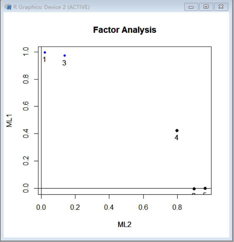
使用factor.plot函数对旋转结果进行可视化:
> factor.plot(fa_model2)
继续渲染,得到一个较为清晰的列表
> fa.diagram(fa_model2, simple = FALSE)
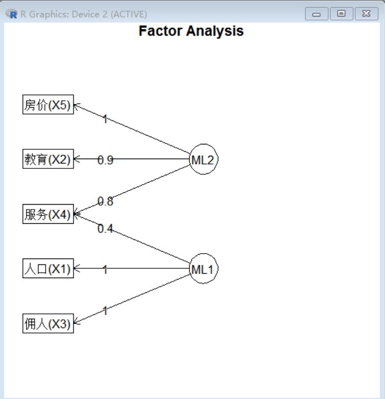
到了这里,我们可以看到,因子1和房价,教育年限和服务人口数相关,可以抽象为经济发展因子,而因子2和人口数,佣人数相关,我们可以抽象成人口规模因子。
以上仅供参考。

这篇关于因子分析的一个小例子的文章就介绍到这儿,希望我们推荐的文章对编程师们有所帮助!