本文主要是介绍curve25519-dalek中field reduce原理分析,希望对大家解决编程问题提供一定的参考价值,需要的开发者们随着小编来一起学习吧!
对于Curve25519,其Field域内的module Fp = 2255-19。
对于64位系统:
/// A `FieldElement51` represents an element of the field
/// \\( \mathbb Z / (2\^{255} - 19)\\).
///
/// In the 64-bit implementation, a `FieldElement` is represented in
/// radix \\(2\^{51}\\) as five `u64`s; the coefficients are allowed to
/// grow up to \\(2\^{54}\\) between reductions modulo \\(p\\).
///
/// # Note
///
/// The `curve25519_dalek::field` module provides a type alias
/// `curve25519_dalek::field::FieldElement` to either `FieldElement51`
/// or `FieldElement2625`.
///
/// The backend-specific type `FieldElement51` should not be used
/// outside of the `curve25519_dalek::field` module.
#[derive(Copy, Clone)]
pub struct FieldElement51(pub (crate) [u64; 5]);
src/backend/serial/u64/field.rs中的reduce函数,是将[u64;5] low-reduce成h, h ∈ [ 0 , 2 ∗ p ) , p = 2 255 − 19 h \in [0, 2*p), p=2^{255}-19 h∈[0,2∗p),p=2255−19。具体的原理如下:
1. field reduce原理分析
如要求某整数 u m o d ( 2 255 − 19 ) u\quad mod \quad (2^{255}-19) umod(2255−19),可将u整数用多项式做如下表示:
u = ∑ i u i 2 51 i x i , 其 中 , u i ∈ N u=\sum_{i}^{}u_i2^{51i}x^i,其中,u_i \in N u=∑iui251ixi,其中,ui∈N
设置x=1,通过对u多项式求值即可代表域Fp内的值。
如需求一个值:
a ∈ [ 0 , 2 320 − 1 ] m o d ( 2 255 − 19 ) = ? a\in [0, 2^{320}-1] \quad mod \quad(2^{255}-19)=? a∈[0,2320−1]mod(2255−19)=?
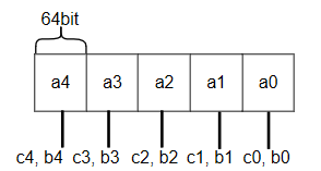
将 a ∈ [ 0 , 2 320 − 1 ] a\in [0, 2^{320}-1] a∈[0,2320−1]以上图表示,同时根据 a i a_i ai分别取相应的 b i , c i b_i,c_i bi,ci:
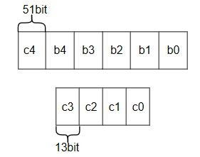
b i = a i & ( 2 < < 51 − 1 ) , c i = a i > > 51 , 其 中 , c i < = 2 13 b_i=a_i \& (2<<51 -1), c_i=a_i >> 51, 其中,c_i<= 2^{13} bi=ai&(2<<51−1),ci=ai>>51,其中,ci<=213
采用parallel carry-out方式进行,对应有:
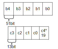
以多项式方式表示时,其中的最高项为:
c 4 ∗ 2 255 ∗ x 5 m o d ( 2 255 − 19 ) c_4*2^{255}*x^5 \quad mod \quad (2^{255}-19) c4∗2255∗x5mod(2255−19)
∵ 2 255 ∗ x 5 ≡ 19 m o d ( 2 255 − 19 ) \because 2^{255}*x^5 \equiv 19 \quad mod \quad (2^{255}-19) ∵2255∗x5≡19mod(2255−19)
∴ c 4 ∗ 2 255 ∗ x 5 ≡ c 4 ∗ 19 m o d ( 2 255 − 19 ) \therefore c_4*2^{255}*x^5 \equiv c_4*19 \quad mod \quad (2^{255}-19) ∴c4∗2255∗x5≡c4∗19mod(2255−19)
所以上图可演化为:
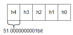
∵ c i < = 2 13 \because c_i<= 2^{13} ∵ci<=213
∵ 2 51 + 2 13 < 2 51 + 2 13 ∗ 19 < 2 51.0000000001 \because 2^{51}+2^{13}<2^{51}+2^{13}*19<2^{51.0000000001} ∵251+213<251+213∗19<251.0000000001
∵ 2 ( 51.0000000001 ∗ 5 ) < 2 ∗ ( 2 255 − 19 ) = 2 ∗ p , p = 2 255 − 19 \because 2^{(51.0000000001*5)} < 2*(2^{255}-19)=2*p, p =2^{255}-19 ∵2(51.0000000001∗5)<2∗(2255−19)=2∗p,p=2255−19
sage: (2^51)+(2^13)*19<2^51.0000000001
True
sage: 2^(51.0000000001*5) < 2*(2^255-19)
True
∴ h 4 = b 4 + c 3 , h 3 = b 3 + c 2 , h 2 = b 2 + c 1 , h 1 = b 1 + c 0 , h 0 = b 0 + c 4 ∗ 19 \therefore h_4=b_4+c_3, h_3=b_3+c_2,h_2=b_2+c_1,h_1=b_1+c_0,h_0=b_0+c_4*19 ∴h4=b4+c3,h3=b3+c2,h2=b2+c1,h1=b1+c0,h0=b0+c4∗19
∴ h = ∑ i = 0 4 h i ∗ 2 ( 51.0000000001 ∗ i ) < 2 ∗ p \therefore h=\sum_{i=0}^{4}h_i*2^{(51.0000000001*i)}<2*p ∴h=∑i=04hi∗2(51.0000000001∗i)<2∗p
2. field reduce代码实现
/// Given 64-bit input limbs, reduce to enforce the bound 2^(51 + epsilon).#[inline(always)]fn reduce(mut limbs: [u64; 5]) -> FieldElement51 {const LOW_51_BIT_MASK: u64 = (1u64 << 51) - 1;// Since the input limbs are bounded by 2^64, the biggest// carry-out is bounded by 2^13.//// The biggest carry-in is c4 * 19, resulting in//// 2^51 + 19*2^13 < 2^51.0000000001//// Because we don't need to canonicalize, only to reduce the// limb sizes, it's OK to do a "weak reduction", where we// compute the carry-outs in parallel.let c0 = limbs[0] >> 51;let c1 = limbs[1] >> 51;let c2 = limbs[2] >> 51;let c3 = limbs[3] >> 51;let c4 = limbs[4] >> 51;limbs[0] &= LOW_51_BIT_MASK;limbs[1] &= LOW_51_BIT_MASK;limbs[2] &= LOW_51_BIT_MASK;limbs[3] &= LOW_51_BIT_MASK;limbs[4] &= LOW_51_BIT_MASK;limbs[0] += c4 * 19;limbs[1] += c0;limbs[2] += c1;limbs[3] += c2;limbs[4] += c3;FieldElement51(limbs)}
3. field reduce结果 ∈ [ 0 , 2 ∗ p ) , p = 2 255 − 19 \in [0, 2*p), p=2^{255}-19 ∈[0,2∗p),p=2255−19
src/backend/serial/u64/field.rs中的sub,neg等函数都只是调用了reduce函数,将最终的返回结果限定在了 ∈ [ 0 , 2 ∗ p ) , p = 2 255 − 19 \in [0, 2*p), p=2^{255}-19 ∈[0,2∗p),p=2255−19,只有调用to_bytes函数,才会将结果限定在 ∈ [ 0 , p ) , p = 2 255 − 19 \in [0, p), p=2^{255}-19 ∈[0,p),p=2255−19。
// -1 + (2^255 - 19) = 2^255 - 20 = p-1let a: [u8;32] = [0xec, 0xff, 0xff, 0xff, 0xff, 0xff, 0xff, 0xff, 0xff, 0xff, 0xff, 0xff, 0xff, 0xff, 0xff, 0xff, 0xff, 0xff, 0xff, 0xff, 0xff, 0xff, 0xff, 0xff, 0xff, 0xff, 0xff, 0xff, 0xff, 0xff, 0xff, 0x7f];let mut b = FieldElement::from_bytes(&a);println!("zyd-before negate b:{:?}", b);b.conditional_negate(Choice::from(1)); //求倒数,用的是reduce结果,对应结果为:-(p-1) mod p = p+1println!("zyd--b:{:?}", b);println!("zyd--b.to_bytes():{:?}", b.to_bytes()); //to_bytes()函数会对结果进行再次module,(p+1) mod p = 1.
对应输出为:
zyd-before negate b:FieldElement51([2251799813685228, 2251799813685247, 2251799813685247, 2251799813685247, 2251799813685247])
zyd--b:FieldElement51([2251799813685230, 2251799813685247, 2251799813685247, 2251799813685247, 2251799813685247])
zyd--b.to_bytes():[1, 0, 0, 0, 0, 0, 0, 0, 0, 0, 0, 0, 0, 0, 0, 0, 0, 0, 0, 0, 0, 0, 0, 0, 0, 0, 0, 0, 0, 0, 0, 0]
4. 一些常量值表示
1)-1对应modulo值为2255-19-1=57896044618658097711785492504343953926634992332820282019728792003956564819948,用FieldElement51表示为:
FieldElement51([2251799813685228, 2251799813685247, 2251799813685247, 2251799813685247, 2251799813685247])
sage: 2251799813685228+2251799813685247*(2^51)+2251799813685247*(2^102)+2251799813685247*(2^153)+2251799813685247*(2^204)==2^255-19-1
True
2)0值对应FieldElement51表示为:
FieldElement51([ 0, 0, 0, 0, 0 ])
3)1值对应FieldElement51表示为:
FieldElement51([ 1, 0, 0, 0, 0 ])
4)16*p值对应FieldElement51表示为:
FieldElement51([ 36028797018963664, 36028797018963952, 36028797018963952, 36028797018963952, 36028797018963952 ])
sage: p=2^255-19
sage: 36028797018963664+36028797018963952*(2^51)+36028797018963952*(2^102)+36028
....: 797018963952*(2^153)+36028797018963952*(2^204)==16*p
True
sage:
这篇关于curve25519-dalek中field reduce原理分析的文章就介绍到这儿,希望我们推荐的文章对编程师们有所帮助!


