本文主要是介绍STK12与Python联合仿真(三):分析星座覆盖性能,希望对大家解决编程问题提供一定的参考价值,需要的开发者们随着小编来一起学习吧!
分析星座覆盖性能
- 打开STK,连接到工程
- 创建种子星 (STK)
- 创建种子星 (Python)
- 生成星座
- Python 创建覆盖网格
- 绑定卫星的传感器
- 建立星座
- 定义多重网格
- 计算与绘图
- 结语
打开STK,连接到工程
jupyter:
导入相关的包
from agi.stk12.stkdesktop import STKDesktop
from agi.stk12.stkobjects import *
from agi.stk12.stkutil import *
from agi.stk12.vgt import *
import os
链接STK
STK_PID = 5600  # 根据自己刚刚得到的PID
stk = STKDesktop.AttachToApplication(pid=int(STK_PID))
# stk = STKDesktop.StartApplication(visible=True) #using optional visible argument
root = stk.Root
print(type(root))
scenario = root.CurrentScenario # 链接当前场景
创建种子星 (STK)
这里我在STK手动建立了高度600km,倾角75° 的种子卫星,并携带了对地观测角80°的传感器
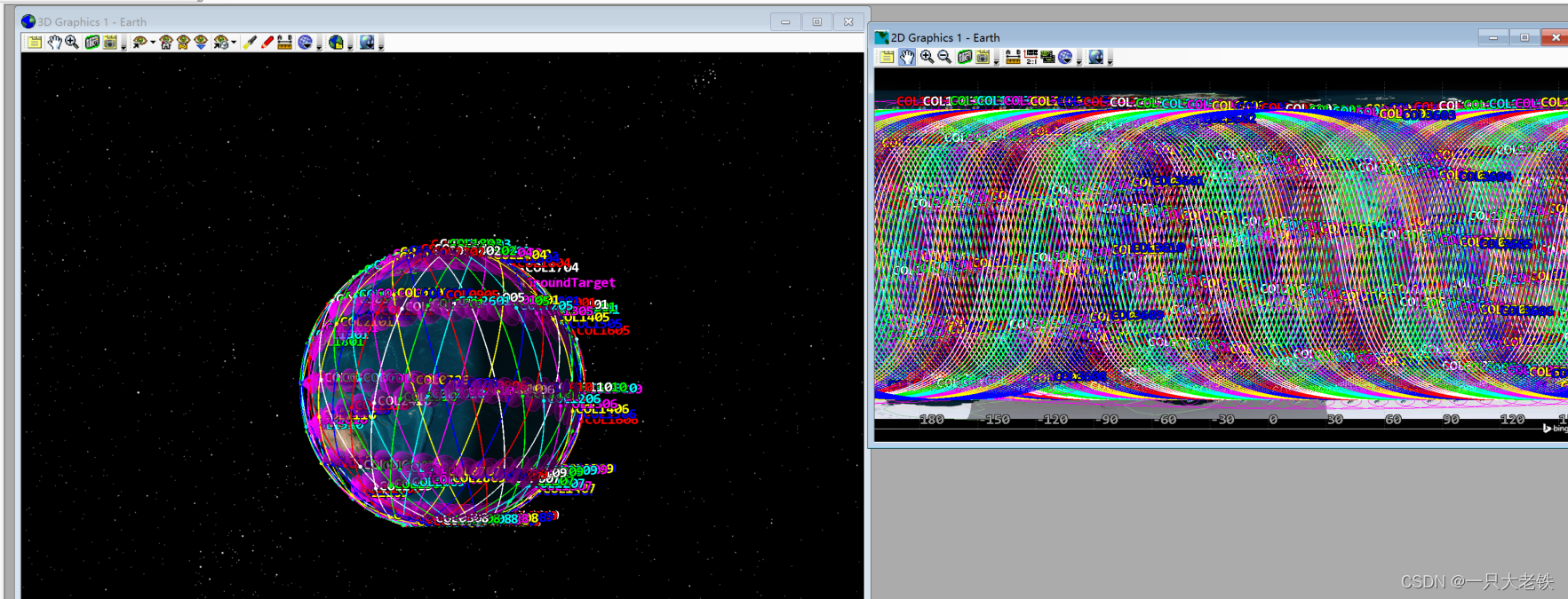
然后建立Wakler星座
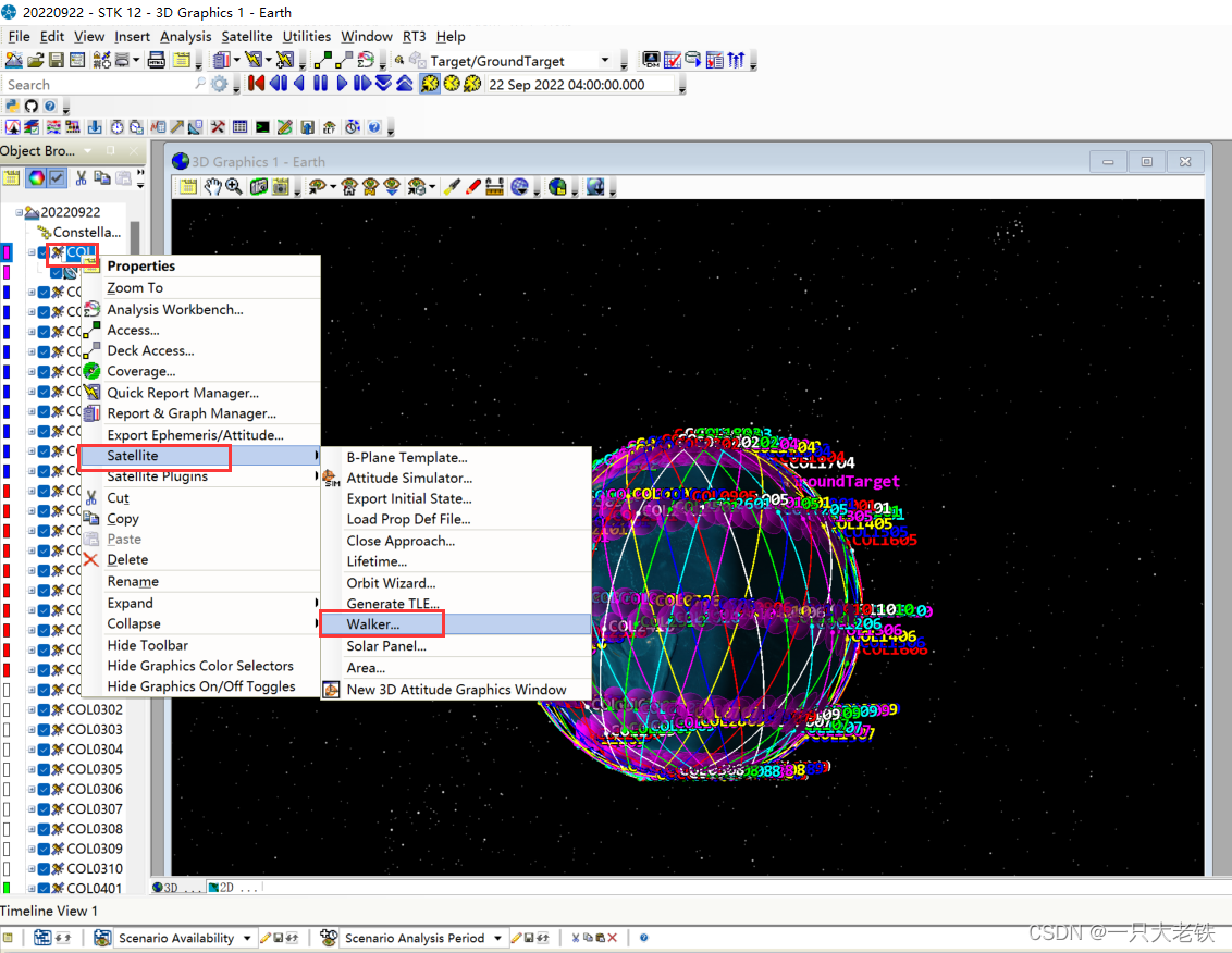
设置36个轨道面,每个轨道面10个星
结果如下:
创建种子星 (Python)
# 创建星座 —— 种子卫星
sat_seed = scenario.Children.New(AgESTKObjectType.eSatellite,'COL') # 种子卫星
# 种子卫星属性
sat_seed.SetPropagatorType(2) #  J4 摄动
keplerian = sat_seed.Propagator.InitialState.Representation.ConvertTo(1)  # eOrbitStateClassical, Use the Classical Element interface
keplerian.SizeShapeType = 0  # eSizeShapeAltitude, Changes from Ecc/Inc to Perigee/Apogee Altitude
keplerian.LocationType = 5  # eLocationTrueAnomaly, Makes sure True Anomaly is being used
keplerian.Orientation.AscNodeType = 0  # eAscNodeLAN, Use LAN instead of RAAN for data entry# Assign the perigee and apogee altitude values:
keplerian.SizeShape.PerigeeAltitude = 600      # km 近地点 高度
keplerian.SizeShape.ApogeeAltitude = 600       # km 远地点 高度# Assign the other desired orbital parameters:
keplerian.Orientation.Inclination = 75         # deg 倾角
keplerian.Orientation.ArgOfPerigee = 0        # deg 近地点幅角度
keplerian.Orientation.AscNode.Value = 0       # deg
keplerian.Location.Value =  0              # deg 平近点角# Apply the changes made to the satellite's state and propagate:
sat_seed.Propagator.InitialState.Representation.Assign(keplerian)
sat_seed.Propagator.Propagate()
- 添加传感器,命名Cam
# 添加传感器
sensor = sat_seed.Children.New(AgESTKObjectType.eSensor,'Cam')
# 传感器属性
sensor.CommonTasks.SetPatternSimpleConic(40,1) # 半张角40°,角分辨率1°
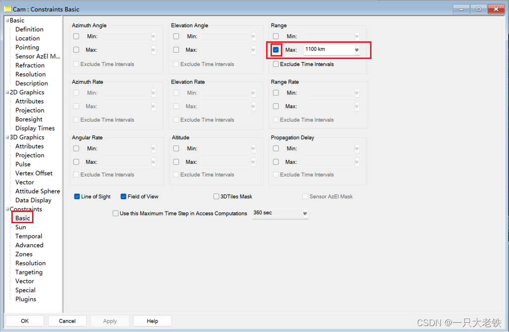
LOS = sensor.AccessConstraints.AddConstraint(34) # Range 类型
# 对照 https://help.agi.com/stkdevkit/Content/DocX/STKObjects~Enumerations~AgEAccessConstraints_EN.html
LOS = LOS.QueryInterface(STKObjects.IAgAccessCnstrMinMax) # 如果报错没有QueryInterface方法就把这一段注释
LOS.EnableMax = True
LOS.Max = 1100
这里解释一下约束
首先https://help.agi.com/stkdevkit/Content/DocX/STKObjectsEnumerationsAgEAccessConstraints_EN.html 这里解释sensor.AccessConstraints.AddConstraint(34)是IAgAccessCnstrMinMax的Range 类型
因此要接入STKObjects.IAgAccessCnstrMinMax,然后LOS.EnableMax对应的是图中的可选框,是否激活
LOS.Max = 1100表示设定的值
比如LOS.EnableMin = True
LOS.Min = 10
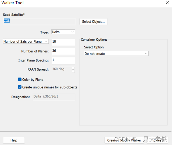
生成星座
生成星座只需要一个命令,
root.ExecuteCommand(‘Walker */Satellite/COL Type Delta NumPlanes 16 NumSatsPerPlane 10 InterPlanePhaseIncrement 1 ColorByPlane Yes’);
在‘Walker */Satellite/COL Type Delta NumPlanes 16 NumSatsPerPlane 10 InterPlanePhaseIncrement 1 ColorByPlane Yes’ 这里面中,COL是种子卫星的平面,往后的参数依次是 轨道平面数、每轨道卫星数、轨道相位因子,对应STK如下
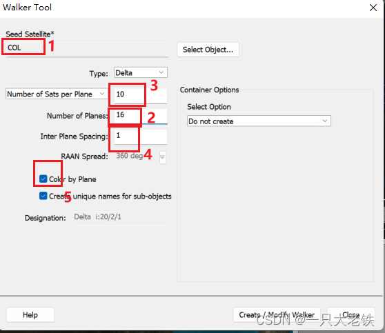
(这里为了演示能快一点就减少了卫星数量)
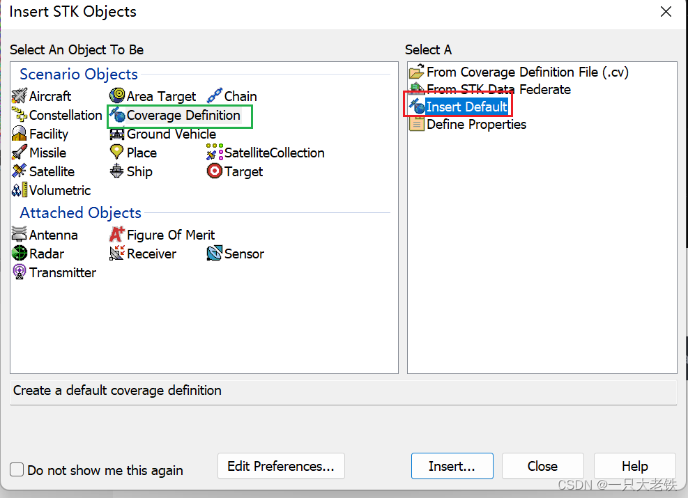
Python 创建覆盖网格
covdef = scenario.Children.New(AgESTKObjectType.eCoverageDefinition,'testCov') # 创建Coverage definition
这里对应STK的
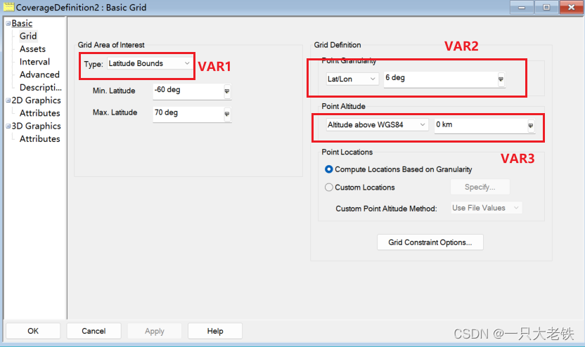
设置 Converage Defination的属性
covdef.Grid.BoundsType = 6 # VAR1
'''
1 Global
2 Latitude Bounds
3 Latitude Line
4 Longitude Line
5 Custom Boundary
6 LatLon Region
'''
covdef.Grid.Resolution.LatLon = 6   # VAR2
covdef.PointDefinition.Altitude = 10 # 10 km  # VAR3# 如果选择eBoundsLatLonRegion可以定义网格的覆盖区域
# covdef.Grid.BoundsType = ‘eBoundsLatLonRegion’;
# covdef.Grid.Bounds.MinLongitude = -120;
# covdef.Grid.Bounds.MaxLongitude = 120;
# covdef.Grid.Bounds.MinLatitude = -30;
# covdef.Grid.Bounds.MaxLatitude = 30;
这里分别对应
绑定卫星的传感器
- 要读取所有可用的对象,放入all_list
- 由于我们只需要卫星的传感器,即放入sensor_list 里面
- 卫星传感器在列表中是交替列出的,因此只要间隔取样就可以了
all_list = covdef.AssetList.AvailableAssets
sensor_list = []
for e in range(len(all_list)):if e%2 == 0:passelse:sensor_list.append(all_list[e])
将所有传感器塞入
for j in sensor_list:covdef.AssetList.Add(j)
建立星座
sate_constellation = scenario.Children.New(AgESTKObjectType.eConstellation,'COL')
for obj in tqdm(all_list):sate_constellation.Objects.Add(obj)
定义多重网格
有时候我们需要分析不同高度的覆盖性能,但是手动添加太过繁琐,一下例程演示0-300km,采样间隔10km的网格创建。
并把不同网格放在一个列表里
covdef_lits = []
for i in range(0,310,10):_string = 'CovDef' + str(i)covdef = scenario.Children.New(AgESTKObjectType.eCoverageDefinition, _string)covdef.Grid.BoundsType = 6covdef.Grid.Resolution.LatLon = 6covdef.PointDefinition.Altitude = i for j in sensor_list:covdef.AssetList.Add(j)covdef_lits.append(covdef)
计算与绘图
| 方法 | 变量值 | 描述 |
|---|---|---|
| eFmAccessConstraint | 0 | Access Constraint Figure of Merit. |
| eFmAccessDuration | 1 | Access Duration Figure of Merit. |
| eFmAccessSeparation | 2 | Access Separation Figure of Merit. |
| eFmCoverageTime | 3 | Coverage Time Figure of Merit. |
| eFmDilutionOfPrecision | 4 | Dilution of Precision Figure of Merit. |
| eFmNAssetCoverage | 5 | N Asset Coverage Figure of Merit. |
| eFmNavigationAccuracy | 6 | Navigation Accuracy Figure of Merit. |
| eFmNumberOfAccesses | 7 | Number of Accesses Figure of Merit. |
| eFmNumberOfGaps | 8 | Number of Gaps Figure of Merit. |
| eFmResponseTime | 9 | Response Time Figure of Merit. |
| eFmRevisitTime | 10 | Revisit Time Figure of Merit. |
| eFmSimpleCoverage | 11 | Simple Coverage Figure of Merit. |
| eFmTimeAverageGap | 12 | Time Average Gap Figure of Merit. |
| eFmSystemResponseTime | 13 | System Response Time Figure of Merit. |
| eFmAgeOfData | 14 | Age of Data Figure of Merit. |
| eFmScalarCalculation | 15 | Scalar Calculation Figure of Merit. |
| eFmSystemAgeOfData | 16 | System Age Of Data Figure of Merit. |
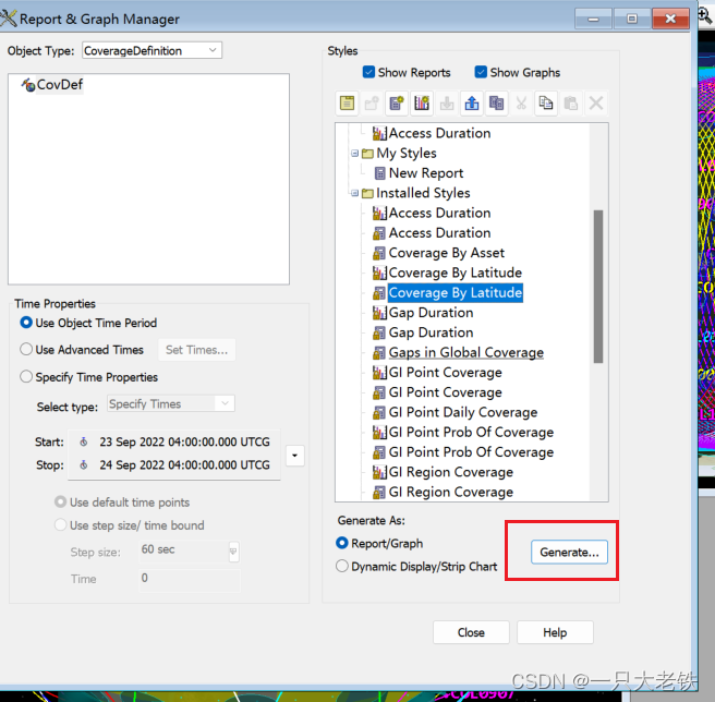
figmerit1.SetDefinitionType(1)  # eFmAccessDuration
covdef_tmp.ComputeAccesses();
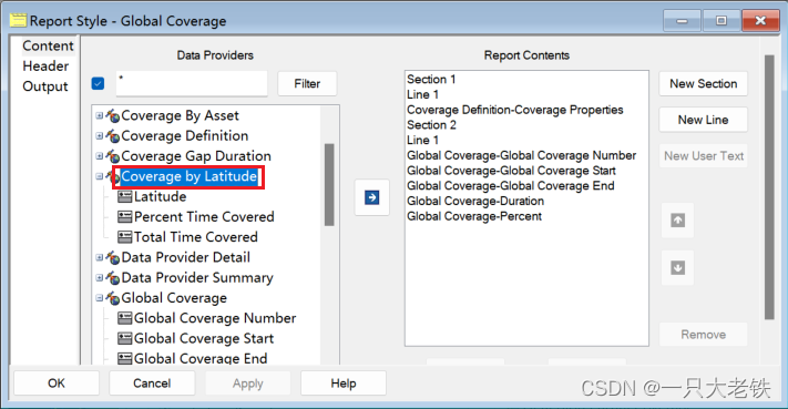
pov = covdef_tmp.DataProviders.Item('Coverage by Latitude').Exec() # Coverage By Latitude
这里对照Reoprt Style 的属性
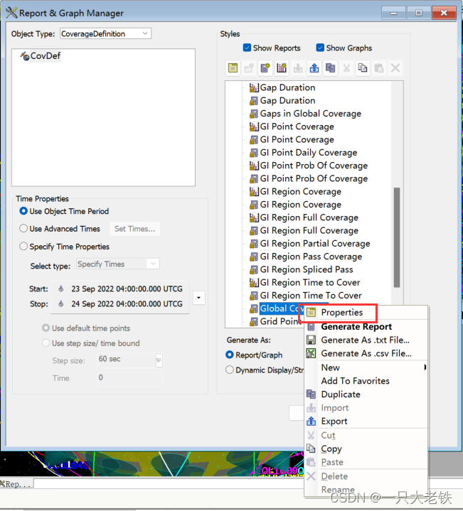
data_array = pov.DataSets.ToArray() # 转换为数组
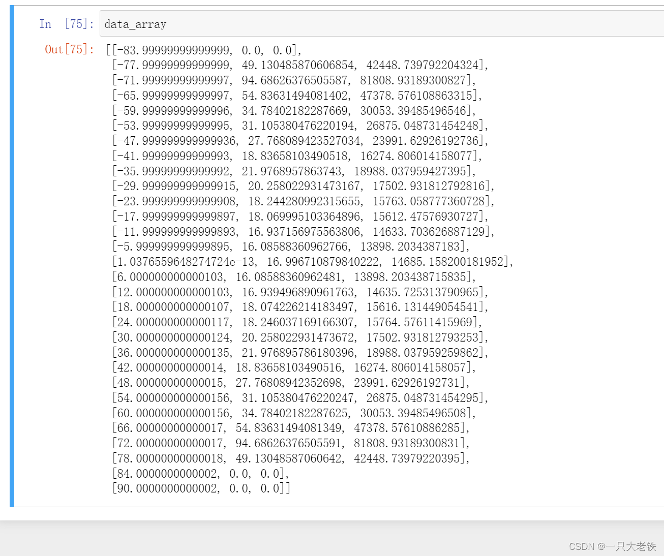
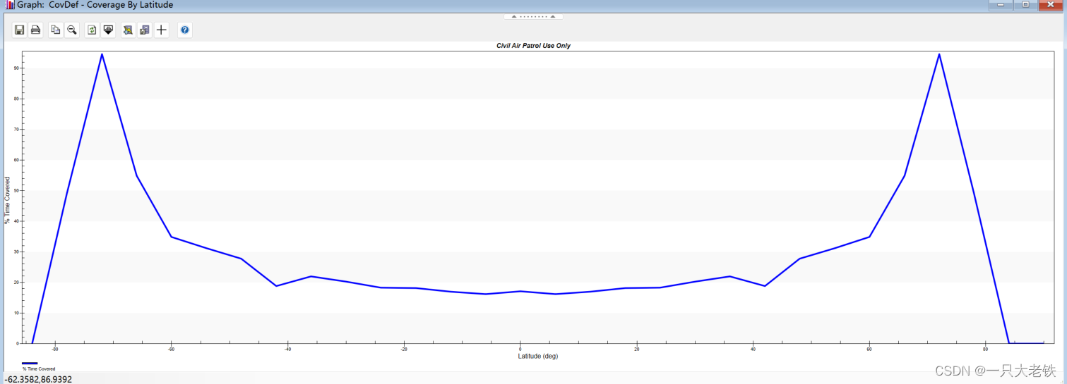
对比STK数据
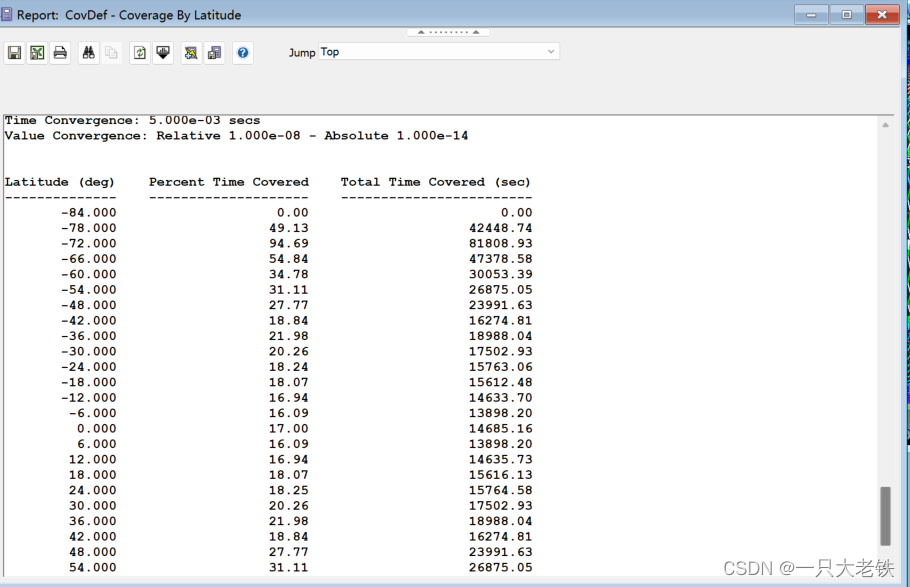
完成绘图
import numpy as np
from matplotlib import pyplot as plt
data_array = np.array(data_array)
x = []
y = []
for ele in data_array:x.append(ele[0])y.append(ele[1])passplt.plot(x,y)
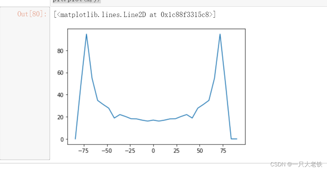
对比STK生成的图
结语
Python 有很多接口都是整形变量,不像MATLAB可以直接用字符串那么方便,需要自己找对应的变量。
我一般是对照着MATLAB的例程找到一些范式,可以在网站中慢慢找
STK Help
本文所有代码我将上传至我的Github
这篇关于STK12与Python联合仿真(三):分析星座覆盖性能的文章就介绍到这儿,希望我们推荐的文章对编程师们有所帮助!


