深入第一个机器学习算法： K-近邻算法(K-Nearest Neighbors)

本文主要是介绍深入第一个机器学习算法： K-近邻算法(K-Nearest Neighbors)，希望对大家解决编程问题提供一定的参考价值，需要的开发者们随着小编来一起学习吧！

本篇博文主要涉及到以下内容：

• K-近邻分类算法
• 从文本文件中解析和导入数据
• 使用Matplotlib创建扩散图
• 归一化数值

K-近邻算法

功能： 非常有效且易于掌握。

学习K-近邻算法的思路：

• 首先，探讨k-近邻算法的基本理论，以及如何使用距离测量的方法分类物品。
• 其次，使用Python 从文本文件中导入并解析数据。
• 再次，讨论当存在多种数据源时，如何避免计算距离时可能碰到的一些常见的错误。
• 最后，利用实际的例子讲解如何使用k-近邻算法改进约会网站和手写数字识别系统。

1.K-近邻算法概述

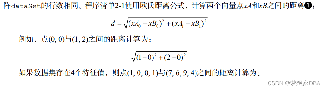
K-近邻算法采用测量不同特征值之间的距离方法进行分类。

k-近邻算法

优点：精度高、对异常值不敏感、无数据输入假定。

缺点：计算复杂度高、空间复杂度高。

适用数据范围：数值型和标称型。

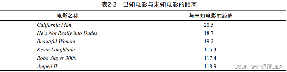
工作原理： 存在一个样本数据集合，也称作训练样本集，并且样本集中每个数据都存在标签，即我们知道样本集中每一数据与所属分类的对应关系。输入没有标签的新数据后，将新数据的每个特征与样本集中数据对应的特征进行比较，然后算法提取样本集中特征最相似数据（最近邻）的分类标签。一般来说，我们只选择样本数据集中前K个最相似的数据，这就是K-邻近算法中K的出处，通常K是不大于20的整数。最后，选择K个最相似数据中出现次数最多的分类，作为新数据的分类。

K-邻近算法的一般流程

1.  收集数据：可以使用任何方法。
2. 准备数据： 距离计算所需要的数值，最好的结构化的数据格式。
3. 分析数据： 可以使用任何方法。
4. 训练算法：此步骤不适用于K-近邻算法。
5. 测试算法： 计算错误率。
6. 使用算法： 首先需要输入样本数据和结构化的输出结果，然后运行K-近邻算法判定输入数据分别属于哪个分类，最后应用对计算出分类执行后续的处理。

2.1.1 准备：使用Python导入数据

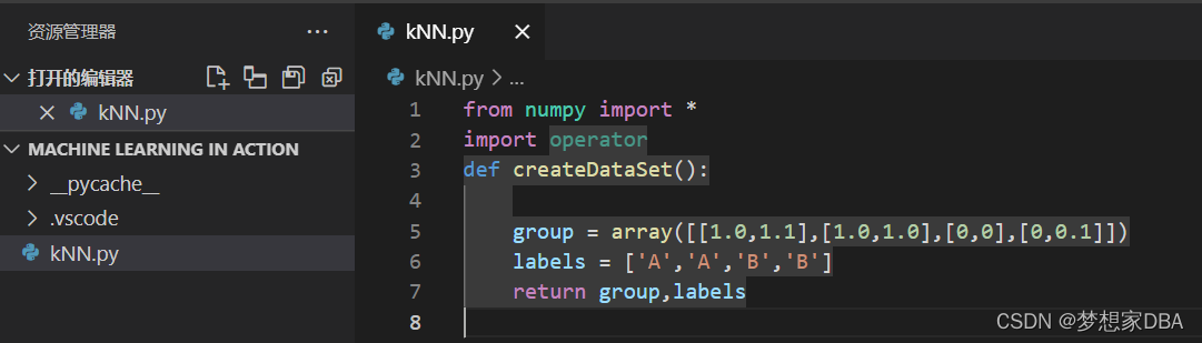
首先创建kNN.py 模块。如下所示：

 code:

from numpy import *

import operator

def createDataSet():

    group = array([[1.0,1.1],[1.0,1.0],[0,0],[0,0.1]])

    labels = ['A','A','B','B']

    return group,labels

以上代码导入了两个模块，科学计算包Numpy，运算符模块

导入程序模块：

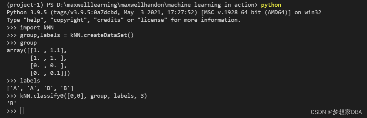
为了确保输入相同的数据集，kNN模块中定义了函数createDataSet.

创建了变量group和labels

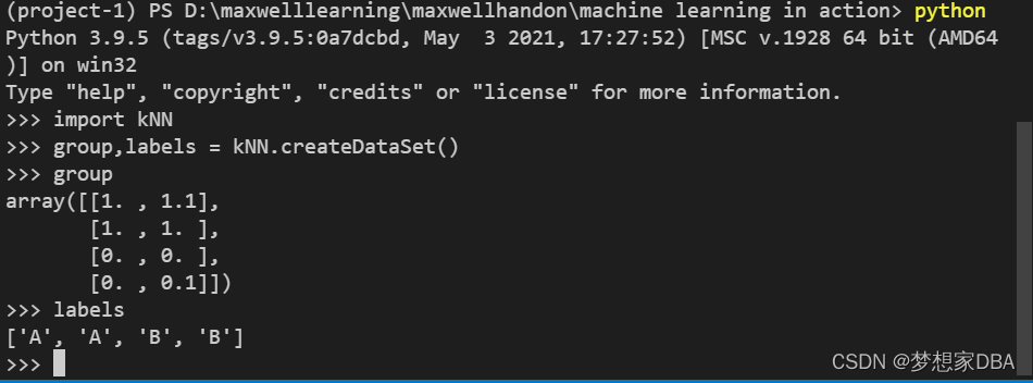
>>> group,labels = kNN.createDataSet()

输入变量的名字以检验是否正确地定义变量：

>>> group
array([[1. , 1.1],
       [1. , 1. ],
       [0. , 0. ],
       [0. , 0.1]])
>>> labels
['A', 'A', 'B', 'B']
>>>

2.1.2 实施kNN算法

对未知类别属性的数据集中的每个点依次执行以下操作：

• 计算已知类别数据集中的点与当前点之间的距离；
• 按照距离递增次序排序。
• 选取与当前点距离最小的k个点。
• 确定前k个点所在类别的出现频率。
• 返回前k个点出现频率最高的类别作为当前点的预测分类。

code:

#   Use k Nearest Neighbors to classify inX accortding to existing dataSet with known ratings in labels

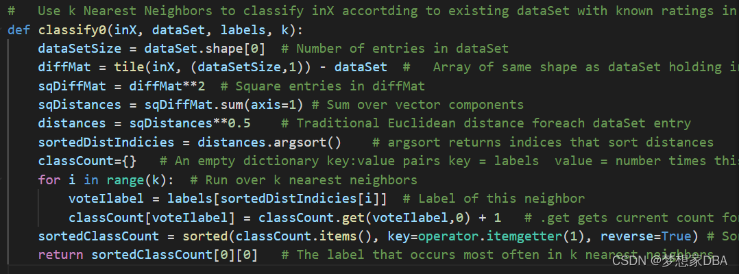
def classify0(inX, dataSet, labels, k):

    dataSetSize = dataSet.shape[0]  # Number of entries in dataSet

    diffMat = tile(inX, (dataSetSize,1)) - dataSet  #   Array of same shape as dataSet holding inX-dataSet entry in each position

    sqDiffMat = diffMat**2  # Square entries in diffMat

    sqDistances = sqDiffMat.sum(axis=1) # Sum over vector components

    distances = sqDistances**0.5    # Traditional Euclidean distance foreach dataSet entry

    sortedDistIndicies = distances.argsort()    # argsort returns indices that sort distances     

    classCount={}   # An empty dictionary key:value pairs key = labels  value = number times this label in set of k       

    for i in range(k):  # Run over k nearest neighbors

        voteIlabel = labels[sortedDistIndicies[i]]  # Label of this neighbor

        classCount[voteIlabel] = classCount.get(voteIlabel,0) + 1   # .get gets current count for voteIlabel and returns zero if first time voteIlabel seen (default = 0)

    sortedClassCount = sorted(classCount.items(), key=operator.itemgetter(1), reverse=True) # Sort classCount (highest to lowest) by voteIlabel count

    return sortedClassCount[0][0]   # The label that occurs most often in k nearest neighbors

classify0() 函数有4个输入参数：

• 用于分类的输入向量是 inX
• 输入的训练样本集为dataSet
• 标签向量为labels
• 最后的参数k表示用于选择最近邻居的数目，其中标签向量的元素数目和矩阵dataSet的行数相同。

 

2.1.3 如何测试分类器

为了测试分类器的效果，我们可以使用已知答案的数据，当然答案不能告诉分类器，检验分 类器给出的结果是否符合预期结果。通过大量的测试数据，我们可以得到分类器的错误率——分 类器给出错误结果的次数除以测试执行的总数。错误率是常用的评估方法，主要用于评估分类器 在某个数据集上的执行效果。完美分类器的错误率为0，最差分类器的错误率是1.0，在这种情况 下，分类器根本就无法找到一个正确答案。

2.2 示例：使用k-近邻算法改进约会网站的配对效果

示例：在约会网站上使用k-近邻算法

(1) 收集数据：提供文本文件。

(2) 准备数据：使用Python解析文本文件。

(3) 分析数据：使用Matplotlib画二维扩散图。

(4) 训练算法：此步骤不适用于k-近邻算法。

(5) 测试算法：使用海伦提供的部分数据作为测试样本。 测试样本和非测试样本的区别在于：测试样本是已经完成分类的数据，如果预测分类 与实际类别不同，则标记为一个错误。

(6) 使用算法：产生简单的命令行程序，然后海伦可以输入一些特征数据以判断对方是否 为自己喜欢的类型。

2.2.1 准备数据： 从文本文件中解析数据

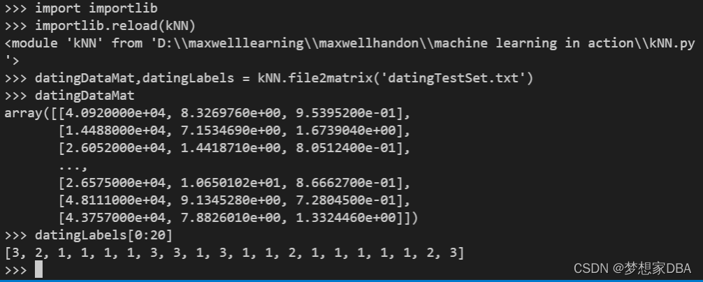
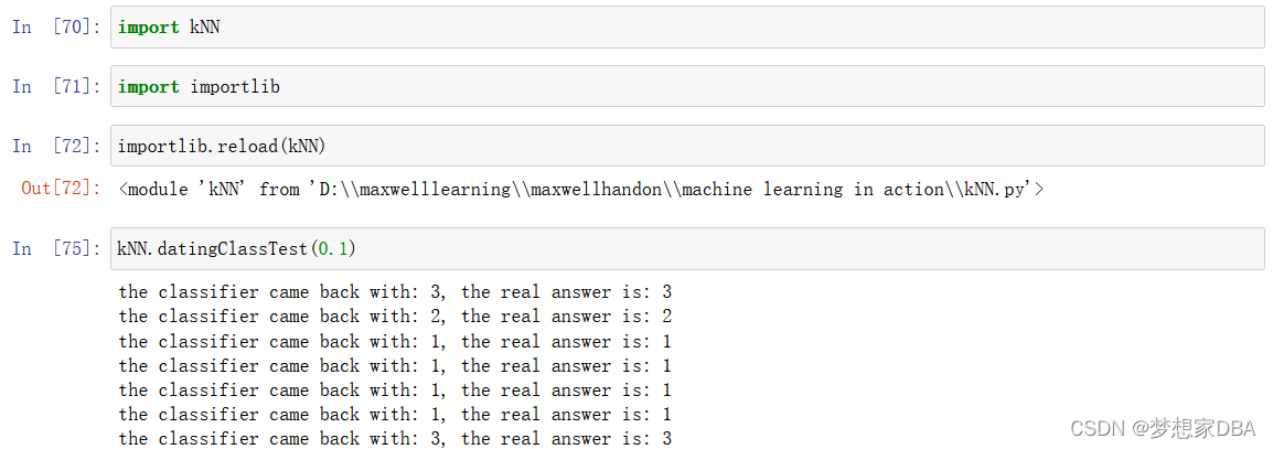
使用函数file2matrix读取文件数据，必须确保文件datingTestSet.txt存储在我们的工作目录中。在执行这个函数之前，需要重新加载一下kNN.py这个模块，以确保更新的内容及时生效。

>>> import kNN
>>> importlib.reload(kNN)
<module 'kNN' from 'D:\\maxwelllearning\\maxwellhandon\\machine learning in action\\kNN.py'>

导入datingTestSet.txt 文件中的数据。

>>> datingDataMat,datingLabels = kNN.file2matrix('datingTestSet.txt')

检测一下数据内容。

>>> datingDataMat
array([[4.0920000e+04, 8.3269760e+00, 9.5395200e-01],
       [1.4488000e+04, 7.1534690e+00, 1.6739040e+00],
       [2.6052000e+04, 1.4418710e+00, 8.0512400e-01],
       ...,
       [2.6575000e+04, 1.0650102e+01, 8.6662700e-01],
       [4.8111000e+04, 9.1345280e+00, 7.2804500e-01],
       [4.3757000e+04, 7.8826010e+00, 1.3324460e+00]])
>>> datingLabels[0:20]
[3, 2, 1, 1, 1, 1, 3, 3, 1, 3, 1, 1, 2, 1, 1, 1, 1, 1, 2, 3]
>>>

 2.2.2 分析数据，使用Matplotlib 创建散点图

首先使用Matplotlib 制作原始数据的散点图。

Code: 

import matplotlib
import matplotlib.pyplot as plt
fig = plt.figure()
ax = fig.add_subplot(111)
ax.scatter(datingDataMat[:,1],datingDataMat[:,2])
plt.show()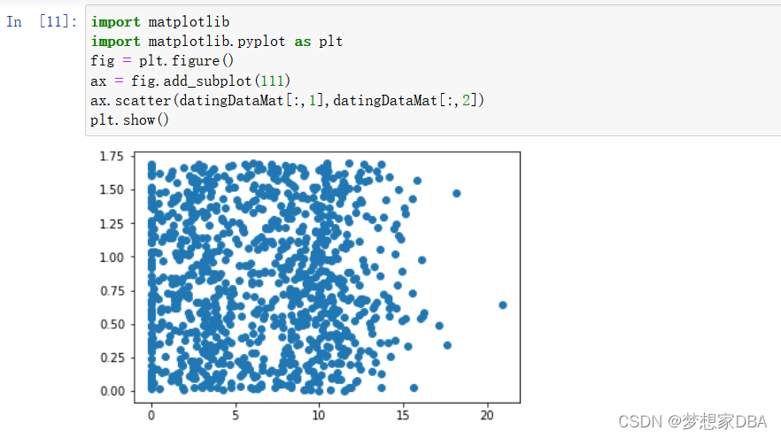

 由于没有使用样本分类的特征值，很难看到任何有用的数据模式信息。一般来说，我们会采用色彩或其他的记号来标记不同样本分类。以便更好地理解数据信息。Matplotlib 库提供的scatter函数支持个性化标记散点图上的点。重新输入上面的代码。调用scatter函数时使用下列参数：

Code:

import matplotlib
from numpy import array
import matplotlib.pyplot as plt
fig = plt.figure()
ax = fig.add_subplot(111)
ax.scatter(datingDataMat[:,1],datingDataMat[:,2], 15.0*array(datingLabels), 15.0*array(datingLabels))
plt.show()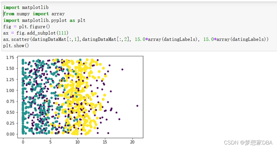

 2.2.3 准备数据：归一化数值

在处理不同取值范围的特征值时，我们通常采用的方法是将数值归一化，如将取值范围处理为０到１或者－１到１之间。下面的公式可以将任意取值范围的特征值转化为０到１区间内的值：

newValue = (oldValue - min)/ (max -min)

其中min和 max 分别是数据集中的最小特征值和最大特征值。故此在kNN.py中增加一个新函数AutoNorm(),该函数可以自动将数字特征值转化为０到１的区间。

# Normalize vector components to be between 0 and 1def autoNorm(dataSet):minVals = dataSet.min(0)maxVals = dataSet.max(0)ranges = maxVals - minValsnormDataSet = zeros(shape(dataSet))m = dataSet.shape[0]normDataSet = dataSet - tile(minVals,(m,1))normDataSet = normDataSet/tile(ranges,(m,1)) #elment wise dividereturn normDataSet, ranges, minVals

２.２.４　测试算法：作为完整程序验证分类器

对于分类器来说，　错误率就是分类器给出错误结果的次数除以测试数据的总数，完成分类器的错误率为０，而错误率为１.０的分类器不会给出任何正确的分类结果。

为了测试分类器效果，在kNN.py 文件中创建函数datingClassTest.该函数是自包含的，你可以在任何时候在Python运行环境中使用该函数测试分类器效果。

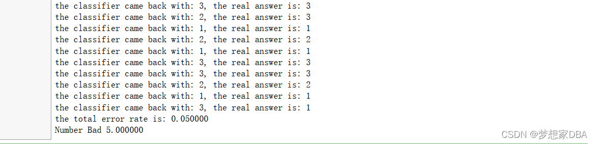
# Use 90% data to predict other 10%. Print fraction of errors
def datingClassTest(hoRatio):# hoRatio is hold out percentagedatingDataMat,datingLabels = file2matrix('datingTestSet.txt')       #load data setfrom filenormMat, ranges, minVals = autoNorm(datingDataMat)m = normMat.shape[0]numTestVecs = int(m*hoRatio)errorCount = 0.0for i in range(numTestVecs):classifierResult = classify0(normMat[i,:],normMat[numTestVecs:m,:],datingLabels[numTestVecs:m],3)print ("the classifier came back with: %d, the real answer is: %d" % (classifierResult, datingLabels[i]))if (classifierResult != datingLabels[i]): errorCount += 1.0print ("the total error rate is: %f" % (errorCount/float(numTestVecs)))print ("Number Bad %f" % errorCount)

输入kNN.datingClassTest(),执行分类器测试程序，我们将得到下面的输出结果：

2.2.5 使用算法：构建完整可用的系统

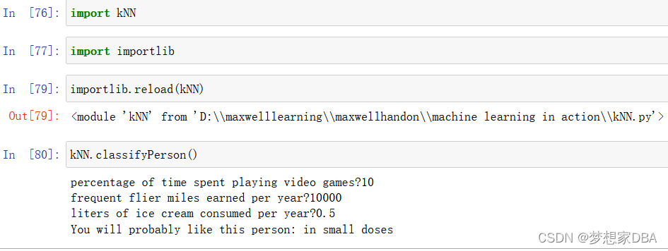
通过给程序海伦会在约会网站上找到某个人并输入他的信息。程序会给出她对对方喜欢程度的预测值。将下列代码加入到kNN.py并重新载入kNN。

Dating site predictor function:

# Dating site predictor function
def classifyPerson():resultList = ['not at all','in small doses','in large doses']percentTats = float(input("percentage of time spent playing video games?"))ffMiles = float(input("frequent flier miles earned per year?"))iceCream = float(input("liters of ice cream consumed per year?"))datingDataMat,datingLabels = file2matrix('datingTestSet.txt')normMat,ranges,minVals = autoNorm(datingDataMat)inArr = array([ffMiles,percentTats,iceCream])classifierResult = classify0((inArr-minVals)/ranges,normMat,datingLabels,3)print("You will probably like this person:",resultList[classifierResult - 1])

This gives the user a text prompt and returns whatever the user enters.

 2.3 Example：a handwriting recognition system

Example: using kNN on a handwriting recognition system

1. Collect: Text file provided.

2. Prepare: Write a function to convert from the image format to the list format used in our classifier, classify0().

3. Analyze: We’ll look at the prepared data in the Python shell to make sure it’s correct.

4. Train: Doesn’t apply to the kNN algorithm.

5. Test: Write a function to use some portion of the data as test examples. The test examples are classified against the non-test examples. If the predicted class doesn’t match the real class, you’ll count that as an error.

6. Use: Not performed in this example. You could build a complete program to extract digits from an image, such a system used to sort the mail in the United States.

2.3.1 Prepare: converting images into test vectors

Convert the image to a vector.The function creates a 1x1024 NumPy array, then opens the given file, loops over the first 32 lines in the file, and stores the integer value of the first 32 characters on each line in the NumPy array. This array is finally returned.

# img2vector converts the image to a vector.
def img2vector(filename):returnVect = zeros((1,1024))fr = open(filename)for i in range(32):lineStr = fr.readline()for j in range(32):returnVect[0,32*i+j] = int(lineStr[j])return returnVect

2.3.2 Test: kNN on handwritten digits

# Handwritten digits testing code
def handwritingClassTest():hwLabels = []trainingFileList = listdir(r'D:\maxwelllearning\maxwellhandon\machine learning in action\trainingDigits')m = len(trainingFileList)trainingMat = zeros((m,1024))for i in range(m):fileNameStr = trainingFileList[i]fileStr = fileNameStr.split('.')[0]classNumStr = int(fileStr.split('_')[0])hwLabels.append(classNumStr)trainingMat[i,:] = img2vector('testDigits/%s' % fileNameStr)testFileList = listdir('testDigits')errorCount = 0.0mTest = len(testFileList)for i in range(mTest):fileNameStr = testFileList[i]fileStr = fileNameStr.split('.')[0]classNumStr = int(fileStr.split('_')[0])vectorUnderTest = img2vector('testDigits/%s' % fileNameStr)classifierResult = classify0(vectorUnderTest, trainingMat, hwLabels, 3)print("the classifier came back with: %d, the real answer is: %d" %(classifierResult, classNumStr))if(classifierResult != classNumStr):errorCount += 1.0print("\nthe total number of errors is: %d" %errorCount)print("\nthe total error rate is: %f" % (errorCount/float(mTest)))

Summary

The k-Nearest Neighbors algorithm is a simple and effective way to classify data. 

An additional drawback is that kNN doesn't give you any idea of the underlying structure of the data; you have no idea what an "average" or "exemplar" instance from each class looks like.

这篇关于深入第一个机器学习算法： K-近邻算法(K-Nearest Neighbors)的文章就介绍到这儿，希望我们推荐的文章对编程师们有所帮助！

---