A tutorial on binary descriptors – part 3 – The ORB descriptor

We’ll start by showing the following figure that shows an example of using ORB to match between real world images with viewpoint change. Green lines are valid matches, red circles indicate unmatched points.

ORB descriptor – An example of keypoints matching using ORB

Now, as you may recall from the previous posts, a binary descriptor is composed out of three parts:

1. A sampling pattern: where to sample points in the region around the descriptor.
2. Orientation compensation: some mechanism to measure the orientation of the keypoint and rotate it to compensate for rotation changes.
3. Sampling pairs: the pairs to compare when building the final descriptor.

Recall that to build the binary string representing a region around a keypoint we need to Go over all the pairs and for each pair (p1, p2) – if the intensity at point p1 is greater than the intensity at point p2, we write 1 in the binary string and 0 otherwise.

The ORB descriptor is a bit similar to BRIEF. It doesn’t have an elaborate sampling pattern as BRISK [3] or FREAK [4]. However, there are two main differences between ORB and BRIEF:

1. ORB uses an orientation compensation mechanism, making it rotation invariant.
2. ORB learns the optimal sampling pairs, whereas BRIEF uses randomly chosen sampling pairs.

Orientation Compensation

ORB uses a simple measure of corner orientation – the intensity centroid [5]. First, the moments of a patch are defined as:

ORB descriptor-Patch’s moments definition

With these moments we can find the centroid, the “center of mass” of the patch as:

ORB descriptor – Center of mass of the patch

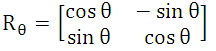
We can construct a vector from the corner’s center O, to the centroid -OC. The orientation of the patch is then given by:

ORB descriptor – Orientation of the patch

Here is an illustration to help explain the method:

ORB descriptor – Angle calculation illustration

Once we’ve calculated the orientation of the patch, we can rotate it to a canonical rotation and then compute the descriptor, thus obtaining some rotation invariance.

我理解一个keypoint周围的patch，应该是以keypoint为中心，的某一个形状。

<1>  在ORB中用灰度质心法求keypoint的方向时，公式里的坐标问题：

第一种理解：以keypoint为坐标原点（0，0）,坐标轴与图像u-o-v坐标轴同向，建立一个局部坐标系。公式里的每个点坐标是在这个坐标系下的坐标，这样求得质心C(cx,cy)的坐标后，与keypoint  O的连线，这个连线与  “ 以keypoint为坐标原点的坐标系” 的X轴的夹角，刚好就是质心C的 arctan(cx,cy)。

第二种理解：公式里的每个点的坐标是在图像坐标系下的，即u-o-v坐标系下的。假设keypoint的坐标为 O（OX,OY）,当用灰度质心法求得这个patch的质心 C（CX, CY）, OC的连线与u轴的夹角为 arctan(CX-OX, CY-OY)。  当图像的灰度确定后，patch的质心位置是确定的，是哪个像素点就是哪个像素点，与在哪个坐标系下计算的无关。所以： keypoint的方向 arctan(cx,cy)=arctan(CX-OX, CY-OY)，因为几何上：cx=CX-OX，cy=CY-OY

<2>ORB 描述子对旋转无关的理解

在光照不变的条件下：当特征点被旋转一个角度 theta后， 特征的方向也被旋转了相应的theta。这就启示我们：如果每一时刻在取patch时的坐标轴与 

特征方向之间的关系是固定不变的，这样当特征点发生旋转时，取的两个patch的像素是完全一样的，两个描述子描述的区域是一样的。

假设在取patch时，先以keypoint为坐标原点（0，0）,坐标轴与图像u-o-v坐标轴同向，取得一个patch S。再对 S进行旋转R(theta),theta为特征的方向，得到一个新的patch S' ， 这个 S’ 是在以keypoint为坐标原点（0，0），x轴与特征的方向同向，y轴与x轴垂直的坐标系下取得的。这样不管特征点怎么旋转，相同特征点的描述子的patch 是同一个区域。即Orientation compensation 的含义。

<3>首先，ORB利用FAST特征点检测的方法来检测特征点，然后利用Harris角点的度量方法，用极大值抑制法，从FAST特征点中挑选出Harris角点响应值最大的 N 个特征点，使得特征点不扎堆，均匀分布，且可以控制特征点的数量。其中Harris角点的响应函数定义为：

R=detM−α(traceM)2

关于 M 的含义和响应函数的由来可以参考Harris角点检测这篇文章。

Learning the sampling pairs

There are two properties we would like our sampling pairs to have.One is uncorrelation – we would like that the sampling pairs will be uncorrelated so that each new pair will bring new information to the descriptor, thus maximizing the amount of information the descriptor carries.The other is high variance of the pairs – high variance makes a feature more discriminative, since it responds differently to inputs.

这一段的思想在这篇中文博客的解释 http://www.cnblogs.com/ronny/p/4083537.html：

ORB使用了一种学习的方法来选择一个较小的点对集合。方法如下：

首先建立一个大约300k关键点的测试集，这些关键点来自于PASCAL2006集中的图像。

对于这300k个关键点中的每一个特征点，考虑它的 31×31 的邻域，我们将在这个邻域内找一些点对。不同于BRIEF中要先对这个Patch内的点做平滑，再用以Patch中心为原点的高斯分布选择点对的方法。ORB为了去除某些噪声点的干扰，选择了一个 5×5 大小的区域的平均灰度来代替原来一个单点的灰度，这里 5×5 区域内图像平均灰度的计算可以用积分图的方法。我们知道 31×31 的Patch里共有 N=(31−5+1)×(31−5+1) 个这种子窗口，那么我们要 N 个子窗口中选择2个子窗口的话，共有 C2N 种方法。所以，对于300k中的每一个特征点，我们都可以从它的 31×31 大小的邻域中提取出一个很长的二进制串，长度为 M=C2N ，表示为

那么当300k个关键点全部进行上面的提取之后，我们就得到了一个 300k×M 的矩阵，矩阵中的每个元素值为0或1。

对该矩阵的每个列向量，也就是每个pair在300k个特征点上的测试结果，计算其均值。把所有的列向量按均值进行重新排序。排好后，组成了一个向量 T ， T 的每一个元素都是一个列向量，列向量其中的元素是每个pair对每个特征点的描述

进行贪婪搜索：从 T 中把排在第一的那个列放到 R 中， T 中就没有这个点对测试结果了。然后把 T 中的排下一个的列与 R 中的所有元素比较，计算它们的相关性，如果相关超过了某一事先设定好的阈值，就扔了它，否则就把它放到 R 里面。重复上面的步骤，只到 R 中有256个列向量为止。如果把 T 完全找完也没有找到256个，那么，可以把相关的阈值调高一些，再重试一遍。

The authors of ORB suggest learning the sampling pairs to ensure they have these two properties. A simple calculation [1] shows that there are about 205,000 possible tests (sampling pairs) to consider. From that vast amount of tests, only 256 tests will be chosen.

The learning is done as follows. First, they set a training set of about 300,000 keypoints drawn from the PASCAL 2006 dataset [6].Next, we apply the following greedy algorithm:

1. Run each test against all training patches.
2. Order the tests by their distance from a mean of 0.5, forming the vector T.
3. Greedy search:
   1. Put the first test into the result vector R and remove it from T.
   2. Take the next test from T, and compare it against all tests in R. If its absolute correlation is greater than a threshold, discard it; else, add it to R.
   3. Repeat the previous step until there are 256 tests in R. If there are fewer than 256, raise the threshold and try again.

Once this algorithm terminates, we obtain a set of 256 relatively uncorrelated tests with high variance.

To conclude, ORB is binary descriptor that is similar to BRIEF, with the added advantages of rotation invariance and learned sampling pairs. You’re probably asking yourself, how does ORB perform in comparison to BRIEF? Well, in non-geometric transformation (those that are image capture dependent and do not rely on the viewpoint, such as blur, JPEG compression, exposure and illumination) BRIEF actually outperforms ORB. In affine transformation, BRIEF perform poorly under large rotation or scale change as it’s not designed to handle such changes. In perspective transformations, which are the result of view-point change, BRIEF surprisingly slightly outperforms ORB. For further details, refer to [7] or wait for the last post in this tutorial which will give a performance evaluation of the binary descriptors.

The next post will talk about BRISK [3] that was actually presented in the same conference as ORB. It presents some difference from BRIEF and ORB by using a hand-crafted sampling pattern.

Gil.

References:

[1] Rublee, Ethan, et al. “ORB: an efficient alternative to SIFT or SURF.” Computer Vision (ICCV), 2011 IEEE International Conference on. IEEE, 2011.‏

[2] Calonder, Michael, et al. “Brief: Binary robust independent elementary features.” Computer Vision–ECCV 2010. Springer Berlin Heidelberg, 2010. 778-792.‏

[3] Leutenegger, Stefan, Margarita Chli, and Roland Y. Siegwart. “BRISK: Binary robust invariant scalable keypoints.” Computer Vision (ICCV), 2011 IEEE International Conference on. IEEE, 2011.‏

[4] Alahi, Alexandre, Raphael Ortiz, and Pierre Vandergheynst. “Freak: Fast retina keypoint.” Computer Vision and Pattern Recognition (CVPR), 2012 IEEE Conference on. IEEE, 2012.‏

[5] Rosin, Paul L. “Measuring corner properties.” Computer Vision and Image Understanding 73.2 (1999): 291-307.‏

[6] M. Everingham. The PASCAL Visual Object Classes Challenge 2006 (VOC2006) Results.http://pascallin.ecs.soton.ac.uk/challenges/VOC/databases.html.

[7] Heinly, Jared, Enrique Dunn, and Jan-Michael Frahm. “Comparative evaluation of binary features.” Computer Vision–ECCV 2012. Springer Berlin Heidelberg, 2012. 759-773.‏