本文主要是介绍深度学习:基于人工神经网络ANN的降雨预测,希望对大家解决编程问题提供一定的参考价值,需要的开发者们随着小编来一起学习吧!

前言
系列专栏:【深度学习:算法项目实战】✨︎
本专栏涉及创建深度学习模型、处理非结构化数据以及指导复杂的模型,如卷积神经网络(CNN)、递归神经网络 (RNN),包括长短期记忆 (LSTM) 、门控循环单元 (GRU)、自动编码器 (AE)、受限玻尔兹曼机(RBM)、深度信念网络 (DBN)、生成对抗网络 (GAN)、深度强化学习(DRL)、大型语言模型(LLM)和迁移学习
降雨预测是对人类社会有重大影响的困难和不确定任务之一。及时准确的预测可以主动帮助减少人员和经济损失。本研究介绍了一组实验,其中涉及使用常见的神经网络技术创建模型,根据澳大利亚主要城市当天的天气数据预测明天是否会下雨。
目录
- 1. 相关库和数据集
- 1.1 相关库介绍
- 1.2 数据集介绍
- 1.3 数据的信息
- 2. 数据可视化和清理
- 2.1 目标列的计数图(检查数据是否平衡)
- 2.2 特征属性之间的相关性
- 2.3 将日期转换为时间序列
- 2.4 将日和月编码为连续循环特征
- 2.5 数据清理——填补缺失值
- 2.5.1 分类变量
- 2.5.2 数值变量
- 2.6 绘制历年降雨量折线图
- 2.7 推算历年阵风风速
- 3. 数据预处理
- 3.1 对分类变量进行编码标签
- 3.2 观察比例特征
- 3.3 观察无离群值的缩放特征
- 4. 模型建立
- 4.1 数据准备(拆分为训练集和测试集)
- 4.2 模型构建
- 4.3 绘制训练和验证损失的Loss曲线
- 4.4 绘制训练和验证的accuracy曲线
- 5. 模型评估
- 5.1 混淆矩阵
- 5.2 分类报告
1. 相关库和数据集
1.1 相关库介绍
Python 库使我们能够非常轻松地处理数据并使用一行代码执行典型和复杂的任务。
Pandas– 该库有助于以 2D 数组格式加载数据框,并具有多种功能,可一次性执行分析任务。Numpy– Numpy 数组速度非常快,可以在很短的时间内执行大型计算。Matplotlib/Seaborn– 此库用于绘制可视化效果,用于展现数据之间的相互关系。Keras– 是一个由Python编写的开源人工神经网络库,可以作为 Tensorflow 的高阶应用程序接口,进行深度学习模型的设计、调试、评估、应用和可视化。
import numpy as np
import pandas as pd
import seaborn as sns
import matplotlib.pyplot as plt
import datetime
from sklearn.preprocessing import LabelEncoder
from sklearn import preprocessing
from sklearn.preprocessing import StandardScaler
from sklearn.model_selection import train_test_splitfrom keras.layers import Dense, BatchNormalization, Dropout, LSTM
from keras.models import Sequential
from keras.utils import to_categorical
from keras.optimizers import Adam
from tensorflow.keras import regularizers
from sklearn.metrics import precision_score, recall_score, confusion_matrix, classification_report, accuracy_score, f1_score
from keras import callbacksnp.random.seed(0)
1.2 数据集介绍
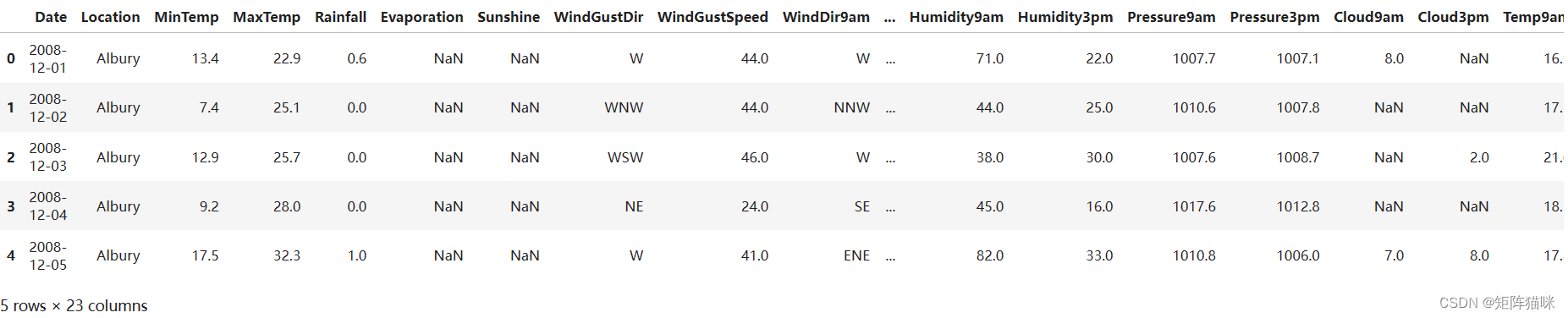
该数据集包含澳大利亚各地约 10 年的每日天气观测数据。观测数据来自众多气象站。在本项目中,我将利用这些数据预测第二天是否会下雨。包括目标变量 "RainTomorrow "在内的 23 个属性表明第二天是否会下雨。
data = pd.read_csv("weatherAUS.csv")
data.head()
1.3 数据的信息
.info()方法打印有关DataFrame的信息,包括索引dtype和列、非null值以及内存使用情况。
data.info()
<class 'pandas.core.frame.DataFrame'>
RangeIndex: 145460 entries, 0 to 145459
Data columns (total 23 columns):#   Column         Non-Null Count   Dtype
---  ------         --------------   -----  0   Date           145460 non-null  object 1   Location       145460 non-null  object 2   MinTemp        143975 non-null  float643   MaxTemp        144199 non-null  float644   Rainfall       142199 non-null  float645   Evaporation    82670 non-null   float646   Sunshine       75625 non-null   float647   WindGustDir    135134 non-null  object 8   WindGustSpeed  135197 non-null  float649   WindDir9am     134894 non-null  object 10  WindDir3pm     141232 non-null  object 11  WindSpeed9am   143693 non-null  float6412  WindSpeed3pm   142398 non-null  float6413  Humidity9am    142806 non-null  float6414  Humidity3pm    140953 non-null  float6415  Pressure9am    130395 non-null  float6416  Pressure3pm    130432 non-null  float6417  Cloud9am       89572 non-null   float6418  Cloud3pm       86102 non-null   float6419  Temp9am        143693 non-null  float6420  Temp3pm        141851 non-null  float6421  RainToday      142199 non-null  object 22  RainTomorrow   142193 non-null  object
dtypes: float64(16), object(7)
memory usage: 25.5+ MB
注意事项:
- 数据集中存在缺失值
- 数据集中包含数值和分类值
2. 数据可视化和清理
2.1 目标列的计数图(检查数据是否平衡)
#first of all let us evaluate the target and find out if our data is imbalanced or not
data.RainTomorrow.value_counts(normalize = True).plot(kind='bar', color= ["#C2C4E2","#EED4E5"], alpha = 0.6, rot=0)

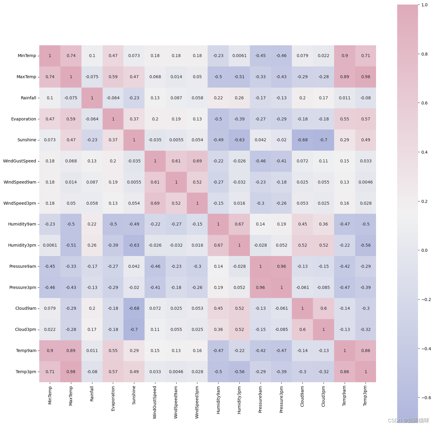
2.2 特征属性之间的相关性
# Correlation amongst numeric attributes
corrmat = data.corr(numeric_only=True)
cmap = sns.diverging_palette(260,-10,s=50, l=75, n=6, as_cmap=True)
plt.subplots(figsize=(18,18))
sns.heatmap(corrmat,cmap= cmap,annot=True, square=True)
2.3 将日期转换为时间序列
我的目标是建立一个人工神经网络(ANN)。我将对日期进行适当的编码,也就是说,我更倾向于将月和日作为一个周期性的连续特征。因为,日期和时间本身就是循环的。为了让 ANN 模型知道某个特征是周期性的,我将其分成周期性的子部分。即年、月和日。现在,我为每个分节创建了两个新特征,分别是分节特征的正弦变换和余弦变换。
#Parsing datetime
#exploring the length of date objects
lengths = data["Date"].str.len()
lengths.value_counts()
Date
10    145460
Name: count, dtype: int64
#There don't seem to be any error in dates so parsing values into datetime
data['Date']= pd.to_datetime(data["Date"])
#Creating a collumn of year
data['year'] = data.Date.dt.year# function to encode datetime into cyclic parameters.
#As I am planning to use this data in a neural network I prefer the months and days in a cyclic continuous feature. def encode(data, col, max_val):data[col + '_sin'] = np.sin(2 * np.pi * data[col]/max_val)data[col + '_cos'] = np.cos(2 * np.pi * data[col]/max_val)return datadata['month'] = data.Date.dt.month
data = encode(data, 'month', 12)data['day'] = data.Date.dt.day
data = encode(data, 'day', 31)
2.4 将日和月编码为连续循环特征
# roughly a year's span section
section = data[:360]
tm = section["day"].plot(color="#C2C4E2")
tm.set_title("Distribution Of Days Over Year")
tm.set_ylabel("Days In month")
tm.set_xlabel("Days In Year")
Text(0.5, 0, 'Days In Year')
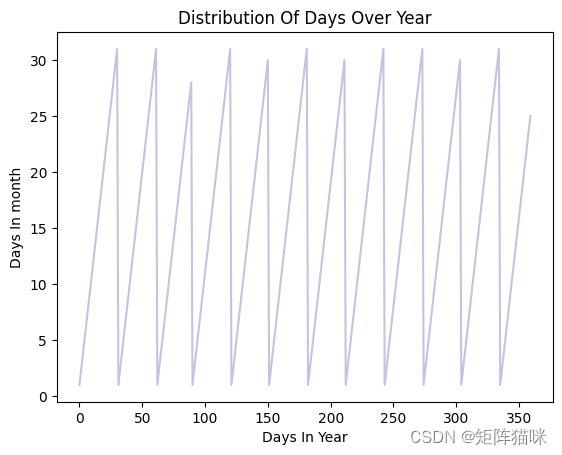
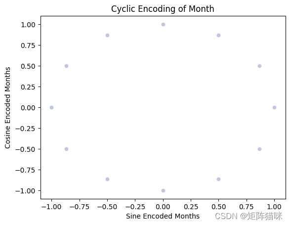
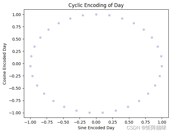
不出所料,数据的 "年份 "属性会重复出现。然而,在这种情况下,真正的周期性并没有以连续的方式呈现出来。将月和日拆分为正弦和余弦组合可提供周期性的连续特征。这可以作为 ANN 的输入特征。
cyclic_month = sns.scatterplot(x="month_sin",y="month_cos",data=data, color="#C2C4E2")
cyclic_month.set_title("Cyclic Encoding of Month")
cyclic_month.set_ylabel("Cosine Encoded Months")
cyclic_month.set_xlabel("Sine Encoded Months")
cyclic_day = sns.scatterplot(x='day_sin',y='day_cos',data=data, color="#C2C4E2")
cyclic_day.set_title("Cyclic Encoding of Day")
cyclic_day.set_ylabel("Cosine Encoded Day")
cyclic_day.set_xlabel("Sine Encoded Day")
接下来,我将分别处理分类属性和数字属性中的缺失值
2.5 数据清理——填补缺失值
2.5.1 分类变量
用列值的众数填补缺失值
# Get list of categorical variables
s = (data.dtypes == "object")
object_cols = list(s[s].index)print("Categorical variables:")
print(object_cols)
Categorical variables:
['Location', 'WindGustDir', 'WindDir9am', 'WindDir3pm', 'RainToday', 'RainTomorrow']
分类变量中的缺失值
# Missing values in categorical variables
for i in object_cols:print(i, data[i].isnull().sum())
Location 0
WindGustDir 10326
WindDir9am 10566
WindDir3pm 4228
RainToday 3261
RainTomorrow 3267
用众数填补缺失值
# Filling missing values with mode of the column in valuefor i in object_cols:data.fillna({i: data[i].mode()[0]}, inplace=True)
2.5.2 数值变量
用列值的中位数填补缺失值
# Get list of neumeric variables
t = (data.dtypes == "float64")
num_cols = list(t[t].index)print("Neumeric variables:")
print(num_cols)
Neumeric variables:
['MinTemp', 'MaxTemp', 'Rainfall', 'Evaporation', 'Sunshine', 'WindGustSpeed', 'WindSpeed9am', 'WindSpeed3pm', 'Humidity9am', 'Humidity3pm', 'Pressure9am', 'Pressure3pm', 'Cloud9am', 'Cloud3pm', 'Temp9am', 'Temp3pm', 'month_sin', 'month_cos', 'day_sin', 'day_cos']
数值变量中的缺失值
# Missing values in numeric variablesfor i in num_cols:print(i, data[i].isnull().sum())
MinTemp 1485
MaxTemp 1261
Rainfall 3261
Evaporation 62790
Sunshine 69835
WindGustSpeed 10263
WindSpeed9am 1767
WindSpeed3pm 3062
Humidity9am 2654
Humidity3pm 4507
Pressure9am 15065
Pressure3pm 15028
Cloud9am 55888
Cloud3pm 59358
Temp9am 1767
Temp3pm 3609
month_sin 0
month_cos 0
day_sin 0
day_cos 0
用列值的中位数填补缺失值
# Filling missing values with median of the column in valuefor i in num_cols:data.fillna({i: data[i].median()}, inplace=True)
data.info()
<class 'pandas.core.frame.DataFrame'>
RangeIndex: 145460 entries, 0 to 145459
Data columns (total 30 columns):#   Column         Non-Null Count   Dtype
---  ------         --------------   -----         0   Date           145460 non-null  datetime64[ns]1   Location       145460 non-null  object        2   MinTemp        145460 non-null  float64       3   MaxTemp        145460 non-null  float64       4   Rainfall       145460 non-null  float64       5   Evaporation    145460 non-null  float64       6   Sunshine       145460 non-null  float64       7   WindGustDir    145460 non-null  object        8   WindGustSpeed  145460 non-null  float64       9   WindDir9am     145460 non-null  object        10  WindDir3pm     145460 non-null  object        11  WindSpeed9am   145460 non-null  float64       12  WindSpeed3pm   145460 non-null  float64       13  Humidity9am    145460 non-null  float64       14  Humidity3pm    145460 non-null  float64       15  Pressure9am    145460 non-null  float64       16  Pressure3pm    145460 non-null  float64       17  Cloud9am       145460 non-null  float64       18  Cloud3pm       145460 non-null  float64       19  Temp9am        145460 non-null  float64       20  Temp3pm        145460 non-null  float64       21  RainToday      145460 non-null  object        22  RainTomorrow   145460 non-null  object        23  year           145460 non-null  int32         24  month          145460 non-null  int32         25  month_sin      145460 non-null  float64       26  month_cos      145460 non-null  float64       27  day            145460 non-null  int32         28  day_sin        145460 non-null  float64       29  day_cos        145460 non-null  float64
dtypes: datetime64[ns](1), float64(20), int32(3), object(6)
memory usage: 31.6+ MB
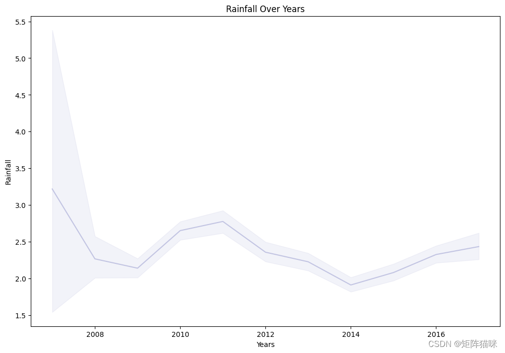
2.6 绘制历年降雨量折线图
#plotting a lineplot rainfall over years
plt.figure(figsize=(12,8))
Time_series=sns.lineplot(x=data['Date'].dt.year,y="Rainfall",data=data,color="#C2C4E2")
Time_series.set_title("Rainfall Over Years")
Time_series.set_ylabel("Rainfall")
Time_series.set_xlabel("Years")
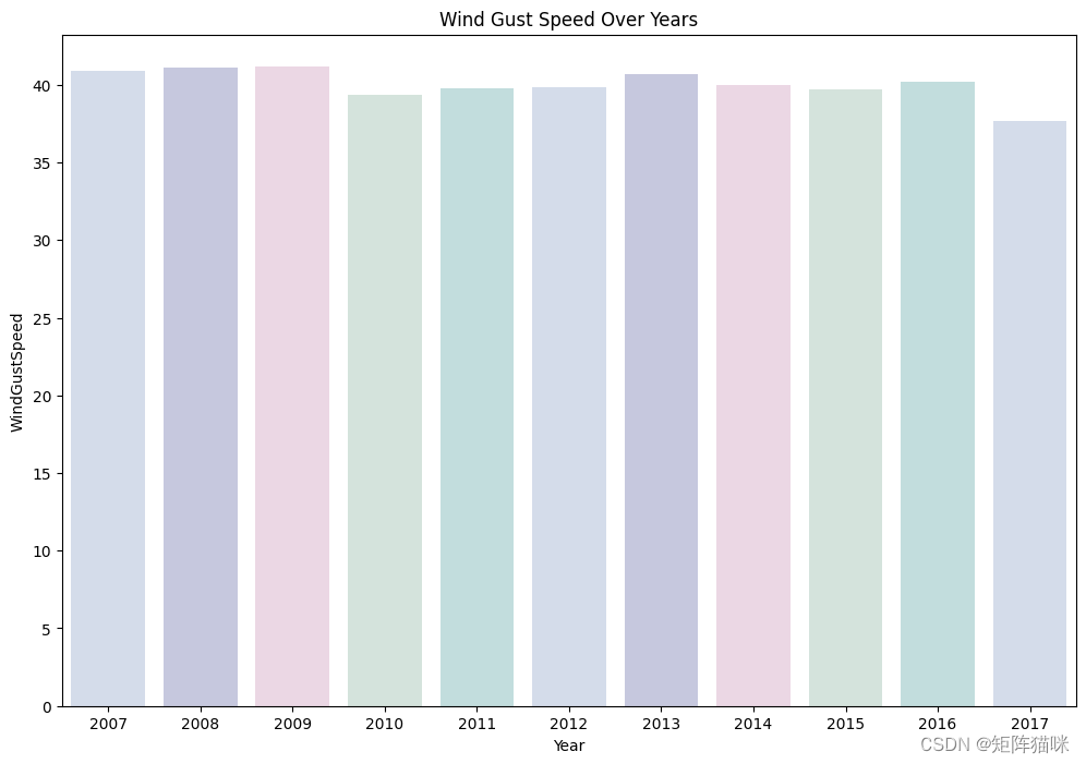
2.7 推算历年阵风风速
#Evauating Wind gust speed over years
colours = ["#D0DBEE", "#C2C4E2", "#EED4E5", "#D1E6DC", "#BDE2E2"]
plt.figure(figsize=(12,8))
Days_of_week=sns.barplot(x=data['Date'].dt.year,y="WindGustSpeed",data=data, errorbar=None, palette = colours)
Days_of_week.set_title("Wind Gust Speed Over Years")
Days_of_week.set_ylabel("WindGustSpeed")
Days_of_week.set_xlabel("Year")
3. 数据预处理
3.1 对分类变量进行编码标签
# Apply label encoder to each column with categorical data
label_encoder = LabelEncoder()
for i in object_cols:data[i] = label_encoder.fit_transform(data[i])
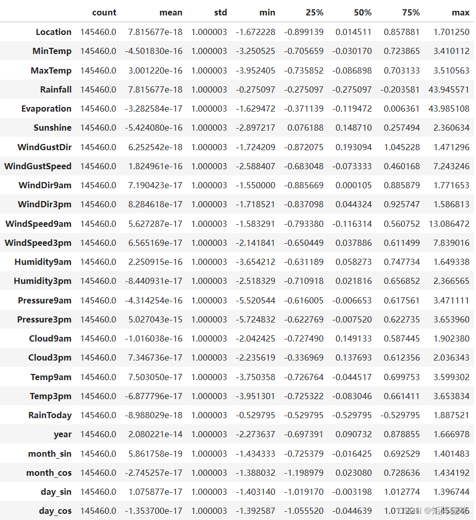
# Prepairing attributes of scale data
features = data.drop(['RainTomorrow', 'Date','day', 'month'], axis=1) # dropping target and extra columns
target = data['RainTomorrow']#Set up a standard scaler for the features
col_names = list(features.columns)
s_scaler = preprocessing.StandardScaler()
features = s_scaler.fit_transform(features)
features = pd.DataFrame(features, columns=col_names) features.describe().T
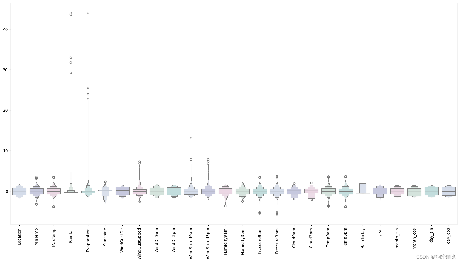
3.2 观察比例特征
#Detecting outliers
#looking at the scaled features
colours = ["#D0DBEE", "#C2C4E2", "#EED4E5", "#D1E6DC", "#BDE2E2"]
plt.figure(figsize=(20,10))
sns.boxenplot(data = features,palette = colours)
plt.xticks(rotation=90)
plt.show()
#full data for
features["RainTomorrow"] = target#Dropping with outlierfeatures = features[(features["MinTemp"]<2.3)&(features["MinTemp"]>-2.3)]
features = features[(features["MaxTemp"]<2.3)&(features["MaxTemp"]>-2)]
features = features[(features["Rainfall"]<4.5)]
features = features[(features["Evaporation"]<2.8)]
features = features[(features["Sunshine"]<2.1)]
features = features[(features["WindGustSpeed"]<4)&(features["WindGustSpeed"]>-4)]
features = features[(features["WindSpeed9am"]<4)]
features = features[(features["WindSpeed3pm"]<2.5)]
features = features[(features["Humidity9am"]>-3)]
features = features[(features["Humidity3pm"]>-2.2)]
features = features[(features["Pressure9am"]< 2)&(features["Pressure9am"]>-2.7)]
features = features[(features["Pressure3pm"]< 2)&(features["Pressure3pm"]>-2.7)]
features = features[(features["Cloud9am"]<1.8)]
features = features[(features["Cloud3pm"]<2)]
features = features[(features["Temp9am"]<2.3)&(features["Temp9am"]>-2)]
features = features[(features["Temp3pm"]<2.3)&(features["Temp3pm"]>-2)]
3.3 观察无离群值的缩放特征
#looking at the scaled features without outliersplt.figure(figsize=(20,10))
sns.boxenplot(data = features,palette = colours)
plt.xticks(rotation=90)
plt.show()
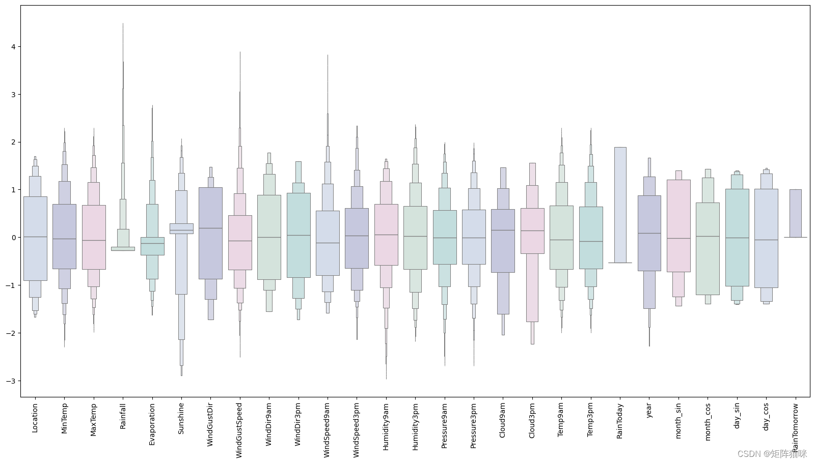
看起来不错,接下来是构建人工神经网络。
4. 模型建立
4.1 数据准备(拆分为训练集和测试集)
X = features.drop(["RainTomorrow"], axis=1)
y = features["RainTomorrow"]# Splitting test and training sets
X_train, X_test,\y_train, y_test = train_test_split(X, y, test_size = 0.2, random_state = 42)
X.shape
(127536, 26)
4.2 模型构建
#Early stopping
early_stopping = callbacks.EarlyStopping(min_delta=0.001, # minimium amount of change to count as an improvementpatience=20, # how many epochs to wait before stoppingrestore_best_weights=True,
)# Initialising the NN
model = Sequential()# layers
model.add(Dense(units = 64, kernel_initializer = 'uniform', activation = 'relu'))
model.add(Dense(units = 32, kernel_initializer = 'uniform', activation = 'relu'))
model.add(Dense(units = 16, kernel_initializer = 'uniform', activation = 'relu'))
model.add(Dropout(0.25))
model.add(Dense(units = 8, kernel_initializer = 'uniform', activation = 'relu'))
model.add(Dropout(0.5))
model.add(Dense(units = 1, kernel_initializer = 'uniform', activation = 'sigmoid'))# Compiling the ANN
opt = Adam(learning_rate=0.00009)
model.compile(optimizer = opt, loss = 'binary_crossentropy', metrics = ['accuracy'])# Train the ANN
history = model.fit(X_train, y_train, batch_size = 32, epochs = 100, callbacks=[early_stopping], validation_split=0.2)
Epoch 1/100
2551/2551 ━━━━━━━━━━━━━━━━━━━━ 4s 937us/step - accuracy: 0.7821 - loss: 0.5575 - val_accuracy: 0.7860 - val_loss: 0.3896
Epoch 2/100
2551/2551 ━━━━━━━━━━━━━━━━━━━━ 2s 882us/step - accuracy: 0.8128 - loss: 0.4126 - val_accuracy: 0.8395 - val_loss: 0.3781
Epoch 3/100
2551/2551 ━━━━━━━━━━━━━━━━━━━━ 2s 875us/step - accuracy: 0.8275 - loss: 0.4005 - val_accuracy: 0.8423 - val_loss: 0.3703
Epoch 4/100
2551/2551 ━━━━━━━━━━━━━━━━━━━━ 2s 922us/step - accuracy: 0.8259 - loss: 0.3985 - val_accuracy: 0.8442 - val_loss: 0.3662
Epoch 5/100
2551/2551 ━━━━━━━━━━━━━━━━━━━━ 2s 876us/step - accuracy: 0.8303 - loss: 0.3930 - val_accuracy: 0.8439 - val_loss: 0.3643
Epoch 6/100
2551/2551 ━━━━━━━━━━━━━━━━━━━━ 2s 885us/step - accuracy: 0.8324 - loss: 0.3905 - val_accuracy: 0.8439 - val_loss: 0.3635
Epoch 7/100
2551/2551 ━━━━━━━━━━━━━━━━━━━━ 2s 918us/step - accuracy: 0.8313 - loss: 0.3906 - val_accuracy: 0.8447 - val_loss: 0.3623
Epoch 8/100
2551/2551 ━━━━━━━━━━━━━━━━━━━━ 2s 888us/step - accuracy: 0.8316 - loss: 0.3888 - val_accuracy: 0.8454 - val_loss: 0.3607
Epoch 9/100
2551/2551 ━━━━━━━━━━━━━━━━━━━━ 2s 921us/step - accuracy: 0.8333 - loss: 0.3876 - val_accuracy: 0.8458 - val_loss: 0.3602
Epoch 10/100
2551/2551 ━━━━━━━━━━━━━━━━━━━━ 3s 911us/step - accuracy: 0.8344 - loss: 0.3836 - val_accuracy: 0.8442 - val_loss: 0.3607
Epoch 11/100
2551/2551 ━━━━━━━━━━━━━━━━━━━━ 2s 891us/step - accuracy: 0.8327 - loss: 0.3841 - val_accuracy: 0.8456 - val_loss: 0.3589
Epoch 12/100
2551/2551 ━━━━━━━━━━━━━━━━━━━━ 2s 881us/step - accuracy: 0.8349 - loss: 0.3838 - val_accuracy: 0.8453 - val_loss: 0.3574
Epoch 13/100
2551/2551 ━━━━━━━━━━━━━━━━━━━━ 2s 907us/step - accuracy: 0.8323 - loss: 0.3846 - val_accuracy: 0.8453 - val_loss: 0.3573
Epoch 14/100
2551/2551 ━━━━━━━━━━━━━━━━━━━━ 2s 883us/step - accuracy: 0.8352 - loss: 0.3817 - val_accuracy: 0.8448 - val_loss: 0.3568
Epoch 15/100
2551/2551 ━━━━━━━━━━━━━━━━━━━━ 2s 936us/step - accuracy: 0.8322 - loss: 0.3827 - val_accuracy: 0.8448 - val_loss: 0.3570
Epoch 16/100
2551/2551 ━━━━━━━━━━━━━━━━━━━━ 2s 878us/step - accuracy: 0.8358 - loss: 0.3803 - val_accuracy: 0.8466 - val_loss: 0.3560
Epoch 17/100
2551/2551 ━━━━━━━━━━━━━━━━━━━━ 3s 928us/step - accuracy: 0.8321 - loss: 0.3809 - val_accuracy: 0.8462 - val_loss: 0.3560
Epoch 18/100
2551/2551 ━━━━━━━━━━━━━━━━━━━━ 3s 938us/step - accuracy: 0.8328 - loss: 0.3832 - val_accuracy: 0.8459 - val_loss: 0.3553
Epoch 19/100
2551/2551 ━━━━━━━━━━━━━━━━━━━━ 2s 877us/step - accuracy: 0.8342 - loss: 0.3763 - val_accuracy: 0.8451 - val_loss: 0.3560
Epoch 20/100
2551/2551 ━━━━━━━━━━━━━━━━━━━━ 3s 913us/step - accuracy: 0.8360 - loss: 0.3758 - val_accuracy: 0.8458 - val_loss: 0.3555
Epoch 21/100
2551/2551 ━━━━━━━━━━━━━━━━━━━━ 3s 893us/step - accuracy: 0.8350 - loss: 0.3780 - val_accuracy: 0.8456 - val_loss: 0.3549
Epoch 22/100
2551/2551 ━━━━━━━━━━━━━━━━━━━━ 2s 893us/step - accuracy: 0.8327 - loss: 0.3794 - val_accuracy: 0.8466 - val_loss: 0.3547
Epoch 23/100
2551/2551 ━━━━━━━━━━━━━━━━━━━━ 3s 899us/step - accuracy: 0.8331 - loss: 0.3791 - val_accuracy: 0.8460 - val_loss: 0.3550
Epoch 24/100
2551/2551 ━━━━━━━━━━━━━━━━━━━━ 2s 905us/step - accuracy: 0.8330 - loss: 0.3785 - val_accuracy: 0.8448 - val_loss: 0.3559
Epoch 25/100
2551/2551 ━━━━━━━━━━━━━━━━━━━━ 2s 880us/step - accuracy: 0.8318 - loss: 0.3790 - val_accuracy: 0.8468 - val_loss: 0.3542
Epoch 26/100
2551/2551 ━━━━━━━━━━━━━━━━━━━━ 3s 904us/step - accuracy: 0.8373 - loss: 0.3709 - val_accuracy: 0.8473 - val_loss: 0.3544
Epoch 27/100
2551/2551 ━━━━━━━━━━━━━━━━━━━━ 3s 948us/step - accuracy: 0.8322 - loss: 0.3800 - val_accuracy: 0.8472 - val_loss: 0.3535
Epoch 28/100
2551/2551 ━━━━━━━━━━━━━━━━━━━━ 2s 892us/step - accuracy: 0.8339 - loss: 0.3791 - val_accuracy: 0.8471 - val_loss: 0.3538
Epoch 29/100
2551/2551 ━━━━━━━━━━━━━━━━━━━━ 2s 917us/step - accuracy: 0.8339 - loss: 0.3755 - val_accuracy: 0.8460 - val_loss: 0.3541
Epoch 30/100
2551/2551 ━━━━━━━━━━━━━━━━━━━━ 2s 882us/step - accuracy: 0.8353 - loss: 0.3748 - val_accuracy: 0.8468 - val_loss: 0.3527
Epoch 31/100
2551/2551 ━━━━━━━━━━━━━━━━━━━━ 3s 901us/step - accuracy: 0.8372 - loss: 0.3712 - val_accuracy: 0.8462 - val_loss: 0.3536
Epoch 32/100
2551/2551 ━━━━━━━━━━━━━━━━━━━━ 2s 901us/step - accuracy: 0.8374 - loss: 0.3741 - val_accuracy: 0.8466 - val_loss: 0.3530
Epoch 33/100
2551/2551 ━━━━━━━━━━━━━━━━━━━━ 2s 877us/step - accuracy: 0.8362 - loss: 0.3740 - val_accuracy: 0.8462 - val_loss: 0.3531
Epoch 34/100
2551/2551 ━━━━━━━━━━━━━━━━━━━━ 2s 899us/step - accuracy: 0.8356 - loss: 0.3746 - val_accuracy: 0.8470 - val_loss: 0.3529
Epoch 35/100
2551/2551 ━━━━━━━━━━━━━━━━━━━━ 2s 880us/step - accuracy: 0.8330 - loss: 0.3754 - val_accuracy: 0.8466 - val_loss: 0.3528
Epoch 36/100
2551/2551 ━━━━━━━━━━━━━━━━━━━━ 2s 875us/step - accuracy: 0.8340 - loss: 0.3767 - val_accuracy: 0.8464 - val_loss: 0.3531
Epoch 37/100
2551/2551 ━━━━━━━━━━━━━━━━━━━━ 2s 924us/step - accuracy: 0.8348 - loss: 0.3743 - val_accuracy: 0.8463 - val_loss: 0.3528
Epoch 38/100
2551/2551 ━━━━━━━━━━━━━━━━━━━━ 2s 876us/step - accuracy: 0.8354 - loss: 0.3758 - val_accuracy: 0.8457 - val_loss: 0.3526
Epoch 39/100
2551/2551 ━━━━━━━━━━━━━━━━━━━━ 2s 919us/step - accuracy: 0.8378 - loss: 0.3698 - val_accuracy: 0.8470 - val_loss: 0.3526
Epoch 40/100
2551/2551 ━━━━━━━━━━━━━━━━━━━━ 2s 886us/step - accuracy: 0.8378 - loss: 0.3741 - val_accuracy: 0.8466 - val_loss: 0.3523
Epoch 41/100
2551/2551 ━━━━━━━━━━━━━━━━━━━━ 2s 894us/step - accuracy: 0.8341 - loss: 0.3770 - val_accuracy: 0.8474 - val_loss: 0.3521
Epoch 42/100
2551/2551 ━━━━━━━━━━━━━━━━━━━━ 2s 883us/step - accuracy: 0.8371 - loss: 0.3708 - val_accuracy: 0.8473 - val_loss: 0.3529
Epoch 43/100
2551/2551 ━━━━━━━━━━━━━━━━━━━━ 2s 880us/step - accuracy: 0.8375 - loss: 0.3743 - val_accuracy: 0.8457 - val_loss: 0.3536
Epoch 44/100
2551/2551 ━━━━━━━━━━━━━━━━━━━━ 3s 929us/step - accuracy: 0.8372 - loss: 0.3709 - val_accuracy: 0.8474 - val_loss: 0.3519
Epoch 45/100
2551/2551 ━━━━━━━━━━━━━━━━━━━━ 3s 907us/step - accuracy: 0.8354 - loss: 0.3722 - val_accuracy: 0.8475 - val_loss: 0.3521
Epoch 46/100
2551/2551 ━━━━━━━━━━━━━━━━━━━━ 3s 905us/step - accuracy: 0.8383 - loss: 0.3709 - val_accuracy: 0.8479 - val_loss: 0.3522
Epoch 47/100
2551/2551 ━━━━━━━━━━━━━━━━━━━━ 2s 893us/step - accuracy: 0.8356 - loss: 0.3752 - val_accuracy: 0.8464 - val_loss: 0.3528
Epoch 48/100
2551/2551 ━━━━━━━━━━━━━━━━━━━━ 2s 882us/step - accuracy: 0.8374 - loss: 0.3707 - val_accuracy: 0.8482 - val_loss: 0.3515
Epoch 49/100
2551/2551 ━━━━━━━━━━━━━━━━━━━━ 2s 909us/step - accuracy: 0.8350 - loss: 0.3745 - val_accuracy: 0.8477 - val_loss: 0.3515
Epoch 50/100
2551/2551 ━━━━━━━━━━━━━━━━━━━━ 3s 911us/step - accuracy: 0.8377 - loss: 0.3720 - val_accuracy:
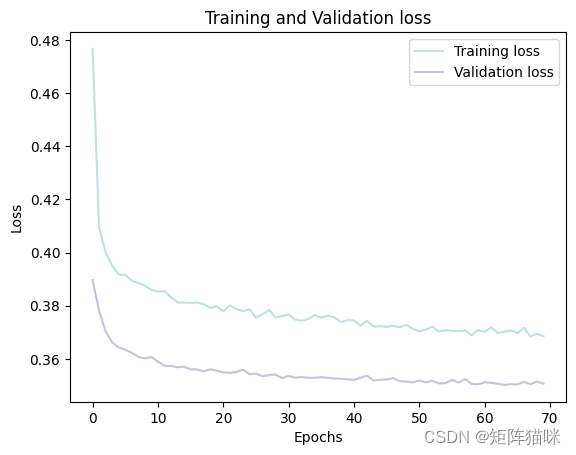
4.3 绘制训练和验证损失的Loss曲线
history_df = pd.DataFrame(history.history)plt.plot(history_df.loc[:, ['loss']], "#BDE2E2", label='Training loss')
plt.plot(history_df.loc[:, ['val_loss']],"#C2C4E2", label='Validation loss')
plt.title('Training and Validation loss')
plt.xlabel('Epochs')
plt.ylabel('Loss')
plt.legend(loc="best")plt.show()
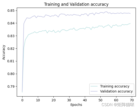
4.4 绘制训练和验证的accuracy曲线
history_df = pd.DataFrame(history.history)plt.plot(history_df.loc[:, ['accuracy']], "#BDE2E2", label='Training accuracy')
plt.plot(history_df.loc[:, ['val_accuracy']], "#C2C4E2", label='Validation accuracy')plt.title('Training and Validation accuracy')
plt.xlabel('Epochs')
plt.ylabel('Accuracy')
plt.legend()
plt.show()
5. 模型评估
预测测试集结果
# Predicting the test set results
y_pred = model.predict(X_test)
y_pred = (y_pred > 0.5)
798/798 ━━━━━━━━━━━━━━━━━━━━ 1s 571us/step
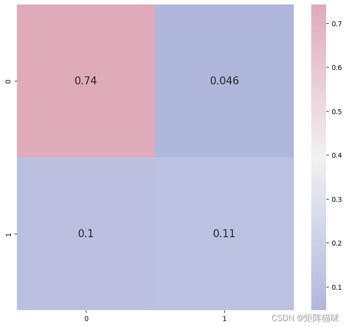
5.1 混淆矩阵
# confusion matrix
cmap1 = sns.diverging_palette(260,-10,s=50, l=75, n=5, as_cmap=True)
plt.subplots(figsize=(9,8))
cf_matrix = confusion_matrix(y_test, y_pred)
sns.heatmap(cf_matrix/np.sum(cf_matrix), cmap = cmap1, annot = True, annot_kws = {'size':15})
5.2 分类报告
print(classification_report(y_test, y_pred))
              precision    recall  f1-score   support0       0.88      0.94      0.91     201101       0.70      0.50      0.59      5398accuracy                           0.85     25508macro avg       0.79      0.72      0.75     25508
weighted avg       0.84      0.85      0.84     25508
这篇关于深度学习:基于人工神经网络ANN的降雨预测的文章就介绍到这儿,希望我们推荐的文章对编程师们有所帮助!


