手把手教你利用 LSTM 模型预测亚马逊股票价格

机器学习是指一套工具或方法，凭借这套工具和方法，利用历史数据对机器进行"训练"进而"学习"到某种模式或规律，并建立预测未来结果的模型。

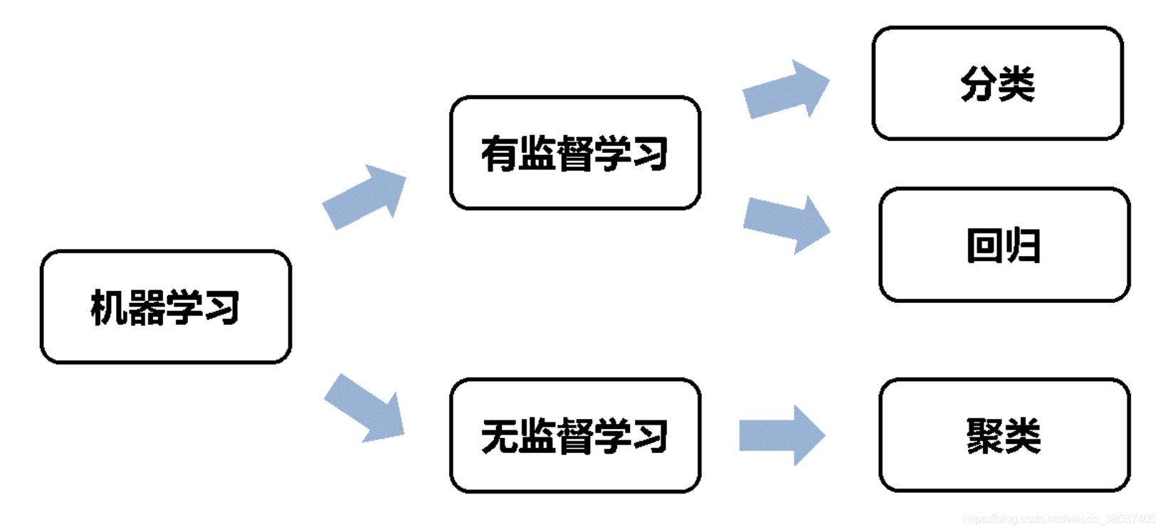
机器学习涉及两类学习方法(如上图):有监督学习，主要用于决策支持，它利用有标识的历史数据进行训练，以实现对新数据的标识的预测。无监督学习方法主要包括聚类。

在日常工作中，预测(回归)是我们经常用到的场景。今天我将手把手分享一个实战项目：如何使用长期记忆(LSTM)预测股票价格。

技术提升

本文由技术群粉丝分享，项目源码、数据、技术交流提升，均可加交流群获取，群友已超过2000人，添加时最好的备注方式为：来源+兴趣方向，方便找到志同道合的朋友

方式①、添加微信号：mlc2060，备注：来自CSDN +研究方向
方式②、微信搜索公众号：机器学习社区，后台回复：加群

LSTM模型

长短期记忆(LSTM)是一种在具有反馈连接的循环神经网络架构。不仅可以处理单个数据点(例如图像)，还可以处理整个数据序列(例如语音或视频)。例如，LSTM适用于诸如未分段，连接的手写识别，语音识别，机器翻译，异常检测，时间序列分析等任务。

LSTM模型的计算量很大，并且需要许多数据。通常，我们使用GPU而不是CPU来训练LSTM模型。Tensorflow是用于训练LSTM模型的强大库。

LSTM股票价格模型

获取数据

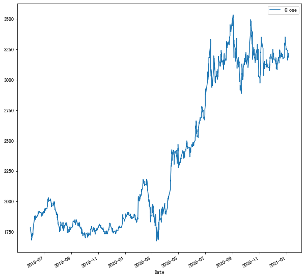
我们将建立一个 LSTM 模型来预测小时股票价格。首先需要加载数据：以亚马逊(AMZN) 股票为例，时间考虑到从’2019–06–01’至’2021–01–07’的每小时收盘价。

import yfinance as yf
import pandas as pd
import numpy as np
import matplotlib.pyplot as plt
%matplotlib inline
data=yf.download('AMZN',start='2019-06-01', interval='1h',  end='2021-01-07',progress=False)[['Close']]
data.head()data.plot(figsize=(10,10))

准备数据

训练数据将具有回溯值作为特征，滞后值为"lb"。对于此示例，我们将lb设置为10。在此示例中，我们将前90％的观测值保留为训练数据集，其余10％作为测试数据集。

from sklearn.preprocessing import MinMaxScaler
cl = data.Close.astype('float32')
train = cl[0:int(len(cl)*0.90)]
scl = MinMaxScaler()
#Scale the data
scl.fit(train.values.reshape(-1,1))
cl =scl.transform(cl.values.reshape(-1,1))
#Create a function to process the data into lb observations look back slices
# and create the train test dataset (90-10)
def processData(data,lb):X,Y = [],[]for i in range(len(data)-lb-1):X.append(data[i:(i+lb),0])Y.append(data[(i+lb),0])return np.array(X),np.array(Y)
lb=10
X,y = processData(cl,lb)
X_train,X_test = X[:int(X.shape[0]*0.90)],X[int(X.shape[0]*0.90):]
y_train,y_test = y[:int(y.shape[0]*0.90)],y[int(y.shape[0]*0.90):]
print(X_train.shape[0],X_train.shape[1])
print(X_test.shape[0],X_test.shape[1])
print(y_train.shape[0])
print(y_test.shape[0])

建立LSTM模型

from keras.layers import LSTM,Dense, Dropout, BatchNormalization
import yfinance as yf
import pandas as pd
import numpy as np
import matplotlib.pyplot as plt
#Build the model
model = Sequential()
model.add(LSTM(256,input_shape=(lb,1)))
model.add(Dense(1))
model.compile(optimizer='adam',loss='mse')
#Reshape data for (Sample,Timestep,Features) 
X_train = X_train.reshape((X_train.shape[0],X_train.shape[1],1))
X_test = X_test.reshape((X_test.shape[0],X_test.shape[1],1))
#Fit model with history to check for overfitting
history = model.fit(X_train,y_train,epochs=300,validation_data=(X_test,y_test),shuffle=False)
model.summary()

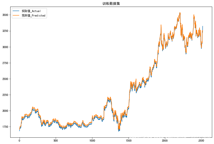
预测

plt.figure(figsize =(12,8))
Xt = model.predict(X_train)
plt.plot(scl.inverse_transform(y_train.reshape(-1,1)),label ="Actual")
plt.plot(scl.inverse_transform(Xt),label ="Predicted")
plt.legend()
plt.title("Train Dataset")

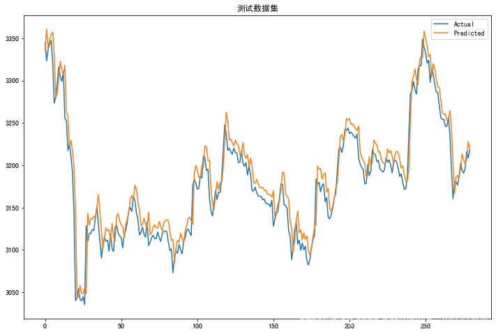
测试

plt.figure(figsize =(12,8))
Xt = model.predict(X_test)
plt.plot(scl.inverse_transform(y_test.reshape(-1,1)),label ="Actual")
plt.plot(scl .inverse_transform(Xt),label ="Predicted")
plt.legend()
plt.title("测试数据集")

评论

该模型可以在训练数据集上完美运行，而在测试数据集上也非常出色。该模型预测单个观测值。在现实场景中，如果我们想预测未来多个预测值，只需调整一下代码即可！