本文主要是介绍[深度学习]Part2 梯度下降法Ch04——【DeepBlue学习笔记】,希望对大家解决编程问题提供一定的参考价值,需要的开发者们随着小编来一起学习吧!
本文仅供学习使用(本章内容与优化方法、凸规划等理论相关,较为简单,相关公式不做具体展开)
梯度下降法Ch04
- 1. 梯度下降法——求θ
- 1.1 随机梯度下降算法(SGD)
- 1.2 批量梯度下降算法(BGD)
- 1.3 小批量梯度下降法(MBGD)
- 1.4 调优策略
- 2. BGD、SGD、MBGD
- 2.1 代码实现
- 2.2 比较
- 2.1 BGD和SGD算法比较
- 2.2 BGD、SGD、MBGD的区别
- 2.3 BGD、SGD、MBGD的比较
1. 梯度下降法——求θ
梯度下降法(Gradient Descent, GD)常用于求解无约束情况下凸函数(Convex Function)的极小值,是一种迭代类型的算法,因为凸函数只有一个极值点,故求解出来的极小值点就是函数的最小值点。
J ( θ ) = 1 2 m ∑ i = 1 m ( h θ ( x ( i ) ) − y ( i ) ) 2 J(\theta )=\frac{1}{2m}\sum\limits_{i=1}^{m}{{{({{h}_{\theta }}({{x}^{(i)}})-{{y}^{(i)}})}^{2}}} J(θ)=2m1i=1∑m(hθ(x(i))−y(i))2(1/m可有可无,对实际结果无影响)
θ ∗ = arg min θ J ( θ ) \theta *=\underset{\theta }{\mathop{\arg \min }}\,J(\theta ) θ∗=θargminJ(θ)
目标函数θ求解 : J ( θ ) = 1 2 ∑ i = 1 m ( h θ ( x ( i ) ) − y ( i ) ) 2 J(\theta )=\frac{1}{2}\sum\limits_{i=1}^{m}{{{({{h}_{\theta }}({{x}^{(i)}})-{{y}^{(i)}})}^{2}}} J(θ)=21i=1∑m(hθ(x(i))−y(i))2
初始化θ(随机初始化,可以初始为0)
沿着负梯度方向迭代,更新后的θ使J(θ)更小: θ ′ = θ − α ∂ J ( θ ) ∂ θ \theta '=\theta -\alpha \frac{\partial J(\theta )}{\partial \theta } θ′=θ−α∂θ∂J(θ),其中α为学习率、步长(学习率大,容易不收敛;学习率小,收敛速度慢)
停止条件——训练数据
仅考虑单个样本的单个θ参数的梯度值:
∂ J ( θ ) ∂ θ j = ∂ ∂ θ j ( 1 2 ( h θ ( x ) − y ) 2 ) = 2 ⋅ 1 2 ( h θ ( x ) − y ) ⋅ ∂ ∂ θ j ( h θ ( x ) − y ) = ( h θ ( x ) − y ) ⋅ ∂ ∂ θ j ( ∑ i = 0 n θ i x i − y ) \frac{\partial J(\theta )}{\partial {{\theta }_{j}}}=\frac{\partial }{\partial {{\theta }_{j}}}(\frac{1}{2}{{({{h}_{\theta }}(x)-y)}^{2}})=2\cdot \frac{1}{2}({{h}_{\theta }}(x)-y)\cdot \frac{\partial }{\partial {{\theta }_{j}}}({{h}_{\theta }}(x)-y)=({{h}_{\theta }}(x)-y)\cdot \frac{\partial }{\partial {{\theta }_{j}}}(\sum\limits_{i=0}^{n}{{{\theta }_{i}}}{{x}_{i}}-y) ∂θj∂J(θ)=∂θj∂(21(hθ(x)−y)2)=2⋅21(hθ(x)−y)⋅∂θj∂(hθ(x)−y)=(hθ(x)−y)⋅∂θj∂(i=0∑nθixi−y)
= ( h θ ( x ) − y ) x j =({{h}_{\theta }}(x)-y){{x}_{j}} =(hθ(x)−y)xj
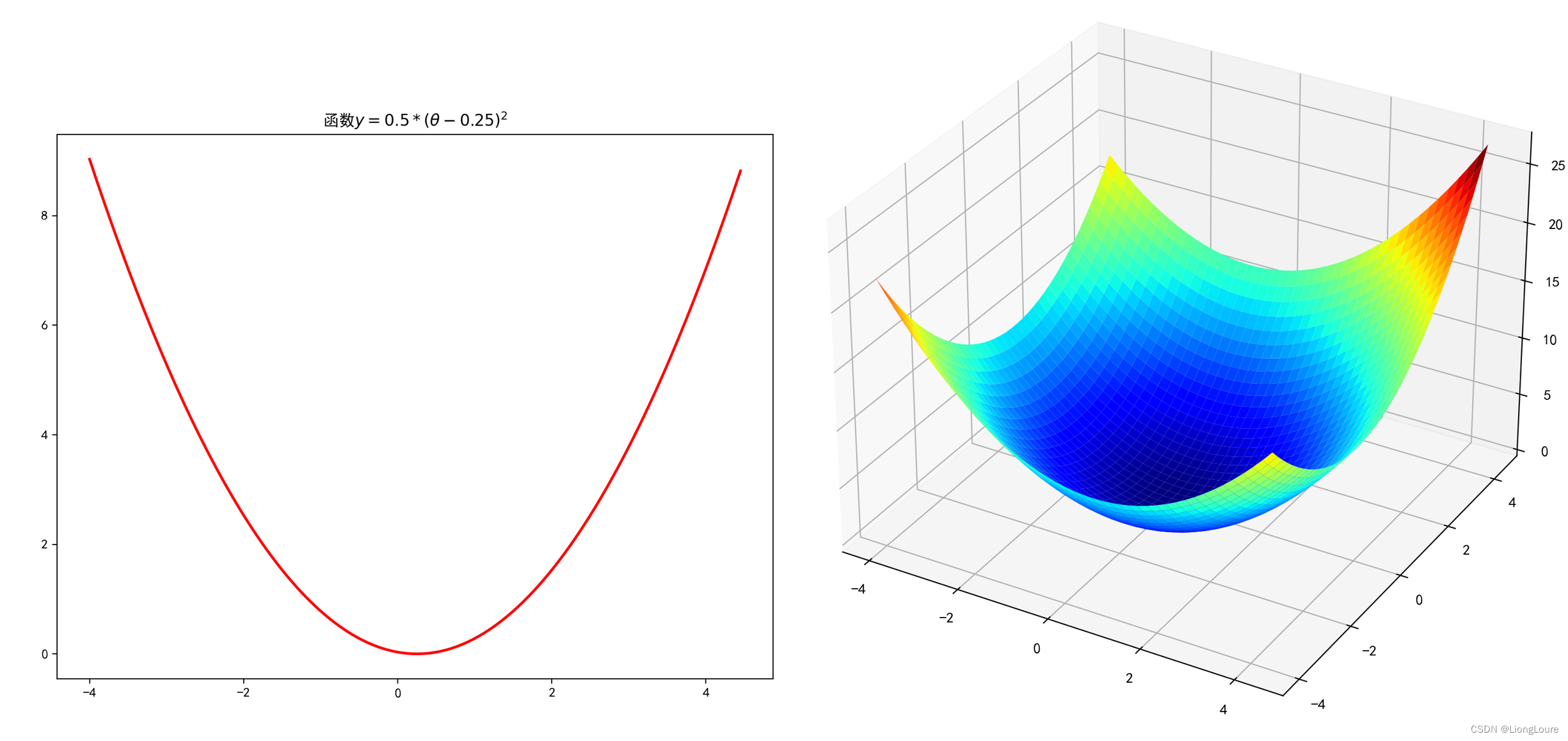
待求解函数:
import numpy as np
import matplotlib as mpl
import matplotlib.pyplot as plt
import math
from mpl_toolkits.mplot3d import Axes3D# 解决中文显示问题
mpl.rcParams['font.sans-serif'] = [u'SimHei']
mpl.rcParams['axes.unicode_minus'] = False# 一维原始图像
def f1(x):return 0.5 * (x - 0.25) ** 2# 构建数据
X = np.arange(-4, 4.5, 0.05)
Y = np.array(list(map(lambda t: f1(t), X)))# 画图
plt.figure(facecolor='w')
plt.plot(X, Y, 'r-', linewidth=2)
plt.title(u'函数$y=0.5 * (θ - 0.25)^2$')
plt.show()# 二维原始图像
def f2(x, y):return 0.6 * (x + y) ** 2 - x * y# 构建数据
X1 = np.arange(-4, 4.5, 0.2)
X2 = np.arange(-4, 4.5, 0.2)
X1, X2 = np.meshgrid(X1, X2)
Y = np.array(list(map(lambda t: f2(t[0], t[1]), zip(X1.flatten(), X2.flatten()))))
Y.shape = X1.shape# 画图
fig = plt.figure(facecolor='w')
ax = Axes3D(fig)
ax.plot_surface(X1, X2, Y, rstride=1, cstride=1, cmap=plt.cm.jet)
ax.set_title(u'函数$y=0.6 * (θ1 + θ2)^2 - θ1 * θ2$')
plt.show()
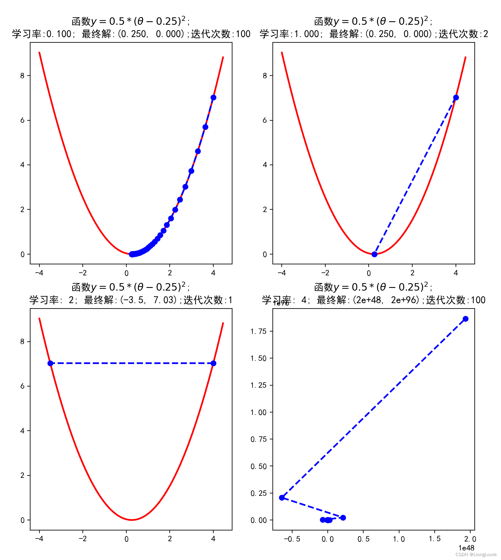
学习率影响
import numpy as np
import matplotlib as mpl
import matplotlib.pyplot as plt
import math
from mpl_toolkits.mplot3d import Axes3D# 解决中文显示问题
mpl.rcParams['font.sans-serif'] = [u'SimHei']
mpl.rcParams['axes.unicode_minus'] = False'''=============================================================================='''# 一维原始图像
def f1(x):return 0.5 * (x - 0.25) ** 2
# 导函数
def h1(x):return 0.5 * 2 * (x - 0.25)# 使用梯度下降法求解
GD_X = []
GD_Y = []
x = 4  # 初始化的x
alpha = 0.1  #步长越小,可能需要的迭代次数就要愈多f_change = 100  # 大于1即可
f_current = f1(x)
GD_X.append(x)
GD_Y.append(f_current)
iter_num = 0
while f_change > 1e-10 and iter_num < 100:  # 停止迭代的条件 差值小于1e-10或者迭代次数大于等于50次iter_num += 1x -= alpha * h1(x)tmp = f1(x)f_change = np.abs(f_current - tmp)f_current  = tmpGD_X.append(x)GD_Y.append(f_current)
# print(u"最终结果为:(%.5f, %.5f)" % (x, f_current))
# print(u"迭代过程中X的取值,迭代次数:%d" % iter_num)
# print(GD_X)# 构建数据
X = np.arange(-4, 4.5, 0.05)
Y = np.array(list(map(lambda t: f1(t), X)))# 画图
plt.figure(facecolor='w')
plt.subplot(2,2,1)
plt.plot(X, Y, 'r-', linewidth=2)
plt.plot(GD_X, GD_Y, 'bo--', linewidth=2)
plt.title(u'函数$y=0.5 * (θ - 0.25)^2$; \n学习率:%.3f; 最终解:(%.3f, %.3f);迭代次数:%d' % (alpha, x, f_current, iter_num))
'''=============================================================================='''
GD_X = []
GD_Y = []
x = 4  # 初始化的x
alpha = 1  #步长越小,可能需要的迭代次数就要愈多f_change = 100  # 大于1即可
f_current = f1(x)
GD_X.append(x)
GD_Y.append(f_current)
iter_num = 0
while f_change > 1e-10 and iter_num < 100:  # 停止迭代的条件 差值小于1e-10或者迭代次数大于等于50次iter_num += 1x -= alpha * h1(x)tmp = f1(x)f_change = np.abs(f_current - tmp)f_current  = tmpGD_X.append(x)GD_Y.append(f_current)
# print(u"最终结果为:(%.5f, %.5f)" % (x, f_current))
# print(u"迭代过程中X的取值,迭代次数:%d" % iter_num)
# print(GD_X)# 构建数据
X = np.arange(-4, 4.5, 0.05)
Y = np.array(list(map(lambda t: f1(t), X)))plt.subplot(2,2,2)
plt.plot(X, Y, 'r-', linewidth=2)
plt.plot(GD_X, GD_Y, 'bo--', linewidth=2)
plt.title(u'函数$y=0.5 * (θ - 0.25)^2$; \n学习率:%.3f; 最终解:(%.3f, %.3f);迭代次数:%d' % (alpha, x, f_current, iter_num))
'''=============================================================================='''
GD_X = []
GD_Y = []
x = 4  # 初始化的x
alpha = 2  #步长越小,可能需要的迭代次数就要愈多f_change = 100  # 大于1即可
f_current = f1(x)
GD_X.append(x)
GD_Y.append(f_current)
iter_num = 0
while f_change > 1e-10 and iter_num < 100:  # 停止迭代的条件 差值小于1e-10或者迭代次数大于等于50次iter_num += 1x -= alpha * h1(x)tmp = f1(x)f_change = np.abs(f_current - tmp)f_current  = tmpGD_X.append(x)GD_Y.append(f_current)
# print(u"最终结果为:(%.5f, %.5f)" % (x, f_current))
# print(u"迭代过程中X的取值,迭代次数:%d" % iter_num)
# print(GD_X)# 构建数据
X = np.arange(-4, 4.5, 0.05)
Y = np.array(list(map(lambda t: f1(t), X)))plt.subplot(2,2,3)
plt.plot(X, Y, 'r-', linewidth=2)
plt.plot(GD_X, GD_Y, 'bo--', linewidth=2)
plt.title(u'函数$y=0.5 * (θ - 0.25)^2$; \n学习率:%2.3g; 最终解:(%2.3g, %2.3g);迭代次数:%d' % (alpha, x, f_current, iter_num))
'''=============================================================================='''GD_X = []
GD_Y = []
x = 4  # 初始化的x
alpha = 4  #步长越小,可能需要的迭代次数就要愈多f_change = 100  # 大于1即可
f_current = f1(x)
GD_X.append(x)
GD_Y.append(f_current)
iter_num = 0
while f_change > 1e-10 and iter_num < 100:  # 停止迭代的条件 差值小于1e-10或者迭代次数大于等于50次iter_num += 1x -= alpha * h1(x)tmp = f1(x)f_change = np.abs(f_current - tmp)f_current  = tmpGD_X.append(x)GD_Y.append(f_current)
# print(u"最终结果为:(%.5f, %.5f)" % (x, f_current))
# print(u"迭代过程中X的取值,迭代次数:%d" % iter_num)
# print(GD_X)# 构建数据
X = np.arange(-4, 4.5, 0.05)
Y = np.array(list(map(lambda t: f1(t), X)))plt.subplot(2,2,4)
plt.plot(X, Y, 'r-', linewidth=2)
plt.plot(GD_X, GD_Y, 'bo--', linewidth=2)
plt.title(u'函数$y=0.5 * (θ - 0.25)^2$; \n学习率:%2.1g; 最终解:(%2.1g, %2.1g);迭代次数:%d' % (alpha, x, f_current, iter_num))
plt.show()
三维
import numpy as np
import matplotlib as mpl
import matplotlib.pyplot as plt
import math
from mpl_toolkits.mplot3d import Axes3D# 二维原始图像
def f2(x, y):return 0.6 * (x + y) ** 2 - x * y
# 导函数
def hx2(x, y):return 0.6 * 2 * (x + y) - y
def hy2(x, y):return 0.6 * 2 * (x + y) - x# 使用梯度下降法求解
GD_X1 = []
GD_X2 = []
GD_Y = []x1 = 4
x2 = 4
alpha = 0.1
f_change = f2(x1, x2)
f_current = f_change
GD_X1.append(x1)
GD_X2.append(x2)
GD_Y.append(f_current)iter_num = 0
while f_change > 1e-10 and iter_num < 100:iter_num += 1prex1 = x1prex2 = x2x1 = x1 - alpha * hx2(prex1, prex2)x2 = x2 - alpha * hy2(prex1, prex2)tmp = f2(x1, x2)f_change = np.abs(f_current - tmp)f_current  = tmpGD_X1.append(x1)GD_X2.append(x2)GD_Y.append(f_current)
print(u"最终结果为:(%.5f, %.5f, %.5f)" % (x1, x2, f_current))
print(u"迭代过程中X的取值,迭代次数:%d" % iter_num)
print(GD_X1)# 构建数据
X1 = np.arange(-4, 4.5, 0.2)
X2 = np.arange(-4, 4.5, 0.2)
X1, X2 = np.meshgrid(X1, X2)
Y = np.array(list(map(lambda t: f2(t[0], t[1]), zip(X1.flatten(), X2.flatten()))))
Y.shape = X1.shape# 画图
fig = plt.figure(facecolor='w')
ax = Axes3D(fig)
ax.plot_surface(X1, X2, Y, rstride=1, cstride=1, cmap=plt.cm.jet)
ax.plot(GD_X1, GD_X2, GD_Y, 'ro--')ax.set_title(u'函数$y=0.6 * (θ1 + θ2)^2 - θ1 * θ2$;\n学习率:%.3f; 最终解:(%.3f, %.3f, %.3f);迭代次数:%d' % (alpha, x1, x2, f_current, iter_num))
plt.show()# 二维原始图像
def f2(x, y):return 0.15 * (x + 0.5) ** 2 + 0.25 * (y  - 0.25) ** 2 + 0.35 * (1.5 * x - 0.2 * y + 0.35 ) ** 2
## 偏函数
def hx2(x, y):return 0.15 * 2 * (x + 0.5) + 0.25 * 2 * (1.5 * x - 0.2 * y + 0.35 ) * 1.5
def hy2(x, y):return 0.25 * 2 * (y  - 0.25) - 0.25 * 2 * (1.5 * x - 0.2 * y + 0.35 ) * 0.2# 使用梯度下降法求解
GD_X1 = []
GD_X2 = []
GD_Y = []
x1 = 4
x2 = 4
alpha = 0.01
f_change = f2(x1, x2)
f_current = f_change
GD_X1.append(x1)
GD_X2.append(x2)
GD_Y.append(f_current)
iter_num = 0
while f_change > 1e-10 and iter_num < 100:iter_num += 1prex1 = x1prex2 = x2x1 = x1 - alpha * hx2(prex1, prex2)x2 = x2 - alpha * hy2(prex1, prex2)tmp = f2(x1, x2)f_change = np.abs(f_current - tmp)f_current  = tmpGD_X1.append(x1)GD_X2.append(x2)GD_Y.append(f_current)
print(u"最终结果为:(%.5f, %.5f, %.5f)" % (x1, x2, f_current))
print(u"迭代过程中X的取值,迭代次数:%d" % iter_num)
print(GD_X1)# 构建数据
X1 = np.arange(-4, 4.5, 0.2)
X2 = np.arange(-4, 4.5, 0.2)
X1, X2 = np.meshgrid(X1, X2)
Y = np.array(list(map(lambda t: f2(t[0], t[1]), zip(X1.flatten(), X2.flatten()))))
Y.shape = X1.shape# 画图
fig = plt.figure(facecolor='w')
ax = Axes3D(fig)
ax.plot_surface(X1, X2, Y, rstride=1, cstride=1, cmap=plt.cm.jet)
ax.plot(GD_X1, GD_X2, GD_Y, 'ko--')
ax.set_xlabel('x')
ax.set_ylabel('y')
ax.set_zlabel('z')ax.set_title(u'函数;\n学习率:%.3f; 最终解:(%.3f, %.3f, %.3f);迭代次数:%d' % (alpha, x1, x2, f_current, iter_num))
plt.show()

1.1 随机梯度下降算法(SGD)
使用单个样本的梯度值作为当前模型参数θ的更新
∂ J ( θ ) ∂ θ j = ( h θ ( x ) − y ) x j \frac{\partial J(\theta )}{\partial {{\theta }_{j}}}=({{h}_{\theta }}(x)-y){{x}_{j}} ∂θj∂J(θ)=(hθ(x)−y)xj
θ j ′ = θ j − α ( h θ ( x ) ( i ) − y ( i ) ) x j ( i ) {{\theta }_{j}}'={{\theta }_{j}}-\alpha ({{h}_{\theta }}{{(x)}^{(i)}}-{{y}^{(i)}}){{x}_{j}}^{(i)} θj′=θj−α(hθ(x)(i)−y(i))xj(i)
每一步迭代需要计算一个方向上的梯度
1.2 批量梯度下降算法(BGD)
使用所有样本的梯度值作为当前模型参数θ的更新
∂ J ( θ ) ∂ θ j = ∑ i = 1 m ( h θ ( x ( i ) ) − y ( i ) ) x j ( i ) \frac{\partial J(\theta )}{\partial {{\theta }_{j}}}=\sum\limits_{i=1}^{m}{({{h}_{\theta }}({{x}^{(i)}})-{{y}^{(i)}})}{{x}_{j}}^{(i)} ∂θj∂J(θ)=i=1∑m(hθ(x(i))−y(i))xj(i)
θ j ′ = θ j − α ∑ i = 1 m ( h θ ( x ( i ) ) − y ( i ) ) x j ( i ) {{\theta }_{j}}'={{\theta }_{j}}-\alpha \sum\limits_{i=1}^{m}{({{h}_{\theta }}({{x}^{(i)}})-{{y}^{(i)}})}{{x}_{j}}^{(i)} θj′=θj−αi=1∑m(hθ(x(i))−y(i))xj(i)
每一步迭代需要计算所有方向上的梯度
1.3 小批量梯度下降法(MBGD)
如果即需要保证算法的训练过程比较快,又需要保证最终参数训练的准确率,而这正是小批量梯度下降法(Mini-batch Gradient Descent,简称 MBGD)的初衷。MBGD中不是每拿一个样本就更新一次梯度,而且拿b 个样本(b一般为10)的平均梯度作为更新方向。
θ j ′ = θ j − α ∑ k = 1 i + 10 ( h θ ( x ( k ) ) − y ( k ) ) x j ( k ) {{\theta }_{j}}'={{\theta }_{j}}-\alpha \sum\limits_{k=1}^{i+10}{({{h}_{\theta }}({{x}^{(k)}})-{{y}^{(k)}})}{{x}_{j}}^{(k)} θj′=θj−αk=1∑i+10(hθ(x(k))−y(k))xj(k)
每一步迭代需要计算10个方向上的梯度
1.4 调优策略
由于梯度下降法中负梯度方向作为变量的变化方向,所以有可能导致最终求解的值是局部最优解,所以在使用梯度下降的时候,一般需要进行一些调优策略:
- 学习率的选择: 学习率过大,表示每次迭代更新的时候变化比较大,有可能会跳过最优解;学习率过小,表示每次迭代更新的时候变化比较小,就会导致迭代速度过慢,很长时间都不能结束;
- 算法初始参数值的选择: 初始值不同,最终获得的最小值也有可能不同,因为梯度下降法求解的是局部最优解,所以一般情况下,选择多次不同初始值运行算法,并最终返回损失函数最小情况下的结果值;
- 标准化: 由于样本不同特征的取值范围不同,可能会导致在各个不同参数上迭代速度不同,为了减少特征取值的影响,可以将特征进行标准化操作。
2. BGD、SGD、MBGD
2.1 代码实现
# encoding=utf-8
import numpy as np
import matplotlib as mpl
import matplotlib.pyplot as plt
import random# 设置字符集,防止中文乱码
mpl.rcParams['font.sans-serif'] = [u'simHei']
mpl.rcParams['axes.unicode_minus'] = False#创建训练数据集
#假设训练学习一个线性函数y = 2.33x
EXAMPLE_NUM = 100 # 训练总数
BATCH_SIZE = 10 # mini_batch训练集大小
TRAIN_STEP = 150 # 训练次数
LEARNING_RATE = 0.0001 # 学习率# 样本
X_INPUT = np.arange(EXAMPLE_NUM) * 0.1 # 生成输入数据X
Y_OUTPUT_CORRECT = 5 * X_INPUT + random.randint(0,1)*np.ones_like(X_INPUT) / 100 # 生成y值##构造训练的函数
def train_func(X, K): # h(theta)result = K * Xreturn result#BGD批量梯度下降算法
#参数初始化值
k_BGD = 0.0
#记录迭代数据用于作图
k_BGD_RECORD = []
for step in range(TRAIN_STEP):SUM_BGD = 0for index in range(len(X_INPUT)):###损失函数J(K)=1/(2m)*sum(KX-y_true)^2###J(K)的梯度 = (KX-y_true)*XSUM_BGD += (train_func(X_INPUT[index], k_BGD) - Y_OUTPUT_CORRECT[index]) * X_INPUT[index]###这里实际上要对SUM_BGD求均值也就是要乘上个1/m 但是 LEARNING_RATE*1/m1 还是一个常数 所以这里就直接用一个常数表示k_BGD -= LEARNING_RATE * SUM_BGDk_BGD_RECORD.append(k_BGD)
# k_BGD_RECORD
print(len(k_BGD_RECORD))# SGD
k_SGD = 0.0
k_SGD_RECORD = []
for step in range(TRAIN_STEP):index = np.random.randint(len(X_INPUT))SUM_SGD = (train_func(X_INPUT[index], k_SGD) - Y_OUTPUT_CORRECT[index]) * X_INPUT[index]k_SGD -= LEARNING_RATE * SUM_SGD # 单个样本梯度k_SGD_RECORD.append(k_SGD)#MBGD
k_MBGD = 0.0
k_MBGD_RECORD = []
for step in range(TRAIN_STEP):SUM_MBGD = 0index_start = np.random.randint(len(X_INPUT) - BATCH_SIZE)for index in np.arange(index_start, index_start+BATCH_SIZE):SUM_MBGD += (train_func(X_INPUT[index], k_MBGD) - Y_OUTPUT_CORRECT[index]) * X_INPUT[index]k_MBGD -= LEARNING_RATE * SUM_MBGDk_MBGD_RECORD.append(k_MBGD)#作图
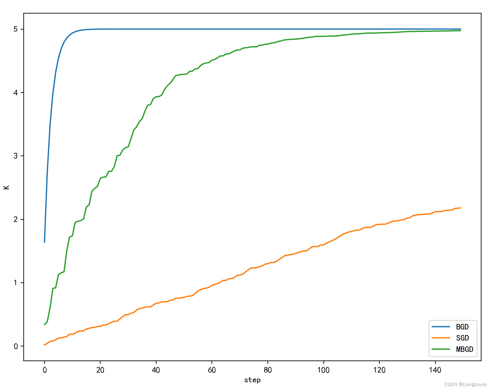
plt.plot(np.arange(TRAIN_STEP), np.array(k_BGD_RECORD), label='BGD')
plt.plot(np.arange(TRAIN_STEP), k_SGD_RECORD, label='SGD')
plt.plot(np.arange(TRAIN_STEP), k_MBGD_RECORD, label='MBGD')
plt.legend()
plt.ylabel('K')
plt.xlabel('step')
plt.show()# SGD
k_SGD = 0.0
k_SGD_RECORD = []
for step in range(TRAIN_STEP*20):index = np.random.randint(len(X_INPUT))SUM_SGD = (train_func(X_INPUT[index], k_SGD) - Y_OUTPUT_CORRECT[index]) * X_INPUT[index]k_SGD -= LEARNING_RATE * SUM_SGDk_SGD_RECORD.append(k_SGD)plt.plot(np.arange(TRAIN_STEP*20), k_SGD_RECORD, label='SGD')
plt.legend()
plt.ylabel('K')
plt.xlabel('step')
plt.show()
2.2 比较
2.1 BGD和SGD算法比较
SGD速度比BGD快(整个数据集从头到尾执行的迭代次数少)
SGD在某些情况下(全局存在多个相对最优解/J(θ)不是一个二次),SGD有可能跳出某些小的局部最优解,所以一般情况下不会比BGD坏;SGD在收敛的位置会存在J(θ)函数波动的情况。
BGD一定能够得到一个局部最优解(在线性回归模型中一定是得到一个全局最优解),SGD由于随机性的存在可能导致最终结果比BGD的差
注意:优先选择SGD
2.2 BGD、SGD、MBGD的区别
- 当样本量为m的时候,每次迭代BGD算法中对于参数值更新一次,SGD算法中对于参数值更新m次,MBGD算法中对于参数值更新m/n次,相对来讲SGD算法的更新速度最快;
- SGD算法中对于每个样本都需要更新参数值,当样本值不太正常的时候,就有可能会导致本次的参数更新会产生相反的影响,也就是说SGD算法的结果并不是完全收敛的,而是在收敛结果处波动的;
- SGD算法是每个样本都更新一次参数值,所以SGD算法特别适合样本数据量大的情况以及在线机器学习(Online ML)。
2.3 BGD、SGD、MBGD的比较
BGD: 可以在迭代步骤上可以快速接近最优解,但是其时间消耗相对其他两种是最大的,因为每一次更新都需要遍历完所有数据。
SGD: 参数更新是最快的,因为每遍历一个数据都会做参数更新,但是由于没有遍历完所有数据,所以其路线不一定是最佳路线,甚至可能会反方向巡迹,不过其整体趋势是往最优解方向行进的,随机速度下降还有一个好处是有一定概率跳出局部最优解,而BGD会直接陷入局部最优解。
MBGD: 以上两种都是MBGD的极端,MBGD是中庸的选择,保证参数更新速度的前提下,用过小批量又增加了其准备度,所以大多数的梯度下降算法中都会使用到小批量梯度下降。
这篇关于[深度学习]Part2 梯度下降法Ch04——【DeepBlue学习笔记】的文章就介绍到这儿,希望我们推荐的文章对编程师们有所帮助!


