MATLAB通过cvx计算L1仿真压缩感知

本文主要是介绍MATLAB通过cvx计算L1仿真压缩感知，希望对大家解决编程问题提供一定的参考价值，需要的开发者们随着小编来一起学习吧！

模拟仿真

下面展示简单的代码：

MATLAB代码

clc;
clearvars;%% Signal Generation
% ------------------
% Define parameters for signal
n = 512;               % Number of samples in the signal
a = 0.2;               % Percentage of the original signal to sample
t = 0:(n-1);           % Time vector% Generate a sparse frequency domain signal using trigonometric functions
f = cos(2*pi/256*t) + sin(2*pi/128*t+2)*5;% Determine the number of samples to keep based on fraction `a`
m = double(int32(a*n));%% Measurement Matrix Generation
% -----------------------------
% Generate the measurement matrix using either a Gaussian or Hadamard matrix
Phi = sqrt(1/m) * randn(m, n);% The sparsity basis matrix (using the inverse FFT)
Psi = inv(fft(eye(n, n)));% The measurement results using the sensing matrix Phi
y = Phi * f';% Matrix A that combines the effects of Phi and Psi
A = Phi * Psi;%% Signal Reconstruction
% ----------------------
% Solve L1-minimization problem using CVX to reconstruct the signal% Start CVX model
cvx_begin;variable x(n) complex;  % Define optimization variable xminimize(norm(x, 1));   % Objective function: Minimize the L1 norm of xsubject toA*x == y;              % Constraint: A*x should be equal to the measurements y
cvx_end;% Obtain the time domain signal from the frequency domain representation
reconstructed_signal = real(ifft(full(x)));%% Visualization
% --------------
% Plot the original and the reconstructed signals
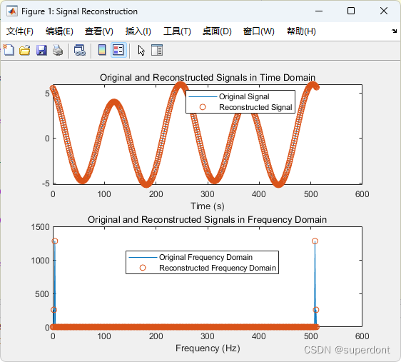
figure('Name', 'Signal Reconstruction');% Original and reconstructed signals in the time domain
subplot(2, 1, 1);
plot(t, f, 'DisplayName', 'Original Signal');
hold on;
plot(t, reconstructed_signal, 'o', 'DisplayName', 'Reconstructed Signal');
hold off;
xlabel('Time (s)');
title('Original and Reconstructed Signals in Time Domain');
legend show;% Original and reconstructed signals in the frequency domain
subplot(2, 1, 2);
plot(t, abs(fft(f)), 'DisplayName', 'Original Frequency Domain');
hold on;
plot(t, abs(x), 'o', 'DisplayName', 'Reconstructed Frequency Domain');
hold off;
xlabel('Frequency (Hz)');
title('Original and Reconstructed Signals in Frequency Domain');
legend show;

输出

信号表达如下：

输出提示：

 
Calling SDPT3 4.0: 1536 variables, 204 equality constraints
------------------------------------------------------------num. of constraints = 204dim. of socp   var  = 1536,   num. of socp blk  = 512
*******************************************************************SDPT3: Infeasible path-following algorithms
*******************************************************************version  predcorr  gam  expon  scale_dataNT      1      0.000   1        0    
it pstep dstep pinfeas dinfeas  gap      prim-obj      dual-obj    cputime
-------------------------------------------------------------------0|0.000|0.000|9.9e-01|2.2e+01|4.2e+05| 1.759155e+04  0.000000e+00| 0:0:00| chol  2  2 1|1.000|0.528|4.4e-08|1.0e+01|4.4e+05| 3.964398e+04  2.596759e+04| 0:0:00| chol  1  1 2|1.000|0.975|4.3e-08|3.4e-01|4.1e+04| 3.325275e+04  3.778379e+03| 0:0:00| chol  1  1 3|0.896|0.733|2.2e-08|1.1e-01|5.7e+03| 8.125834e+03  3.388853e+03| 0:0:00| chol  1  1 4|0.950|1.000|6.6e-09|7.8e-03|9.5e+02| 4.003548e+03  3.084480e+03| 0:0:01| chol  1  1 5|0.983|0.983|1.4e-10|2.4e-03|1.6e+01| 3.087983e+03  3.079534e+03| 0:0:01| chol  1  1 6|0.955|0.986|1.8e-10|7.2e-04|7.2e-01| 3.072707e+03  3.074302e+03| 0:0:01| chol  2  1 7|0.843|1.000|4.8e-09|2.1e-04|1.7e-01| 3.072165e+03  3.072671e+03| 0:0:01| chol  2  2 8|0.948|0.985|2.5e-10|3.2e-06|9.4e-03| 3.072009e+03  3.072010e+03| 0:0:01| chol  2  2 9|0.969|0.987|6.7e-10|4.2e-08|3.0e-04| 3.072000e+03  3.072000e+03| 0:0:01| chol  3  3 
10|0.994|1.000|2.6e-10|7.6e-11|6.3e-06| 3.072000e+03  3.072000e+03| 0:0:01|stop: max(relative gap, infeasibilities) < 1.49e-08
-------------------------------------------------------------------number of iterations   = 10primal objective value =  3.07200001e+03dual   objective value =  3.07200000e+03gap := trace(XZ)       = 6.30e-06relative gap           = 1.03e-09actual relative gap    = 1.01e-09rel. primal infeas (scaled problem)   = 2.55e-10rel. dual     "        "       "      = 7.56e-11rel. primal infeas (unscaled problem) = 0.00e+00rel. dual     "        "       "      = 0.00e+00norm(X), norm(y), norm(Z) = 2.6e+03, 5.4e+01, 2.3e+01norm(A), norm(b), norm(C) = 2.4e+00, 7.7e+01, 2.4e+01Total CPU time (secs)  = 0.99  CPU time per iteration = 0.10  termination code       =  0DIMACS: 9.0e-10  0.0e+00  8.9e-10  0.0e+00  1.0e-09  1.0e-09
-------------------------------------------------------------------------------------------------------------------------------
Status: Solved
Optimal value (cvx_optval): +3072>> 

参考资料：

压缩感知的实现（含matlab代码）

原文中实现了多种形式，本程序对其进行了裁剪。

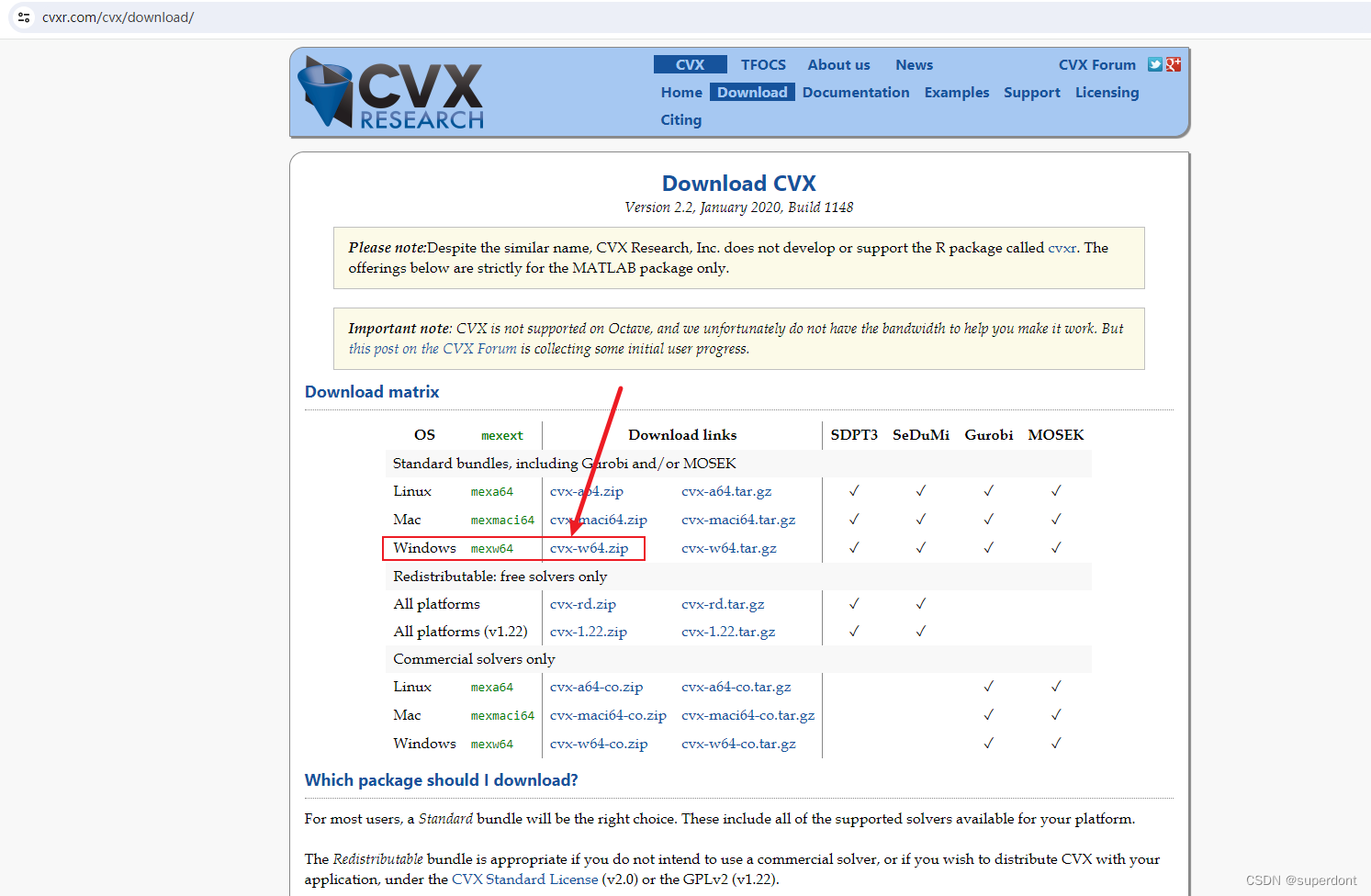
CVX下载

网址：
https://cvxr.com/cvx/

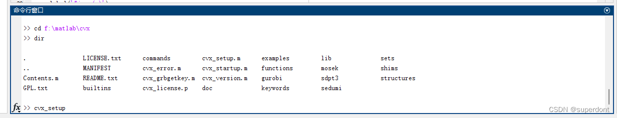
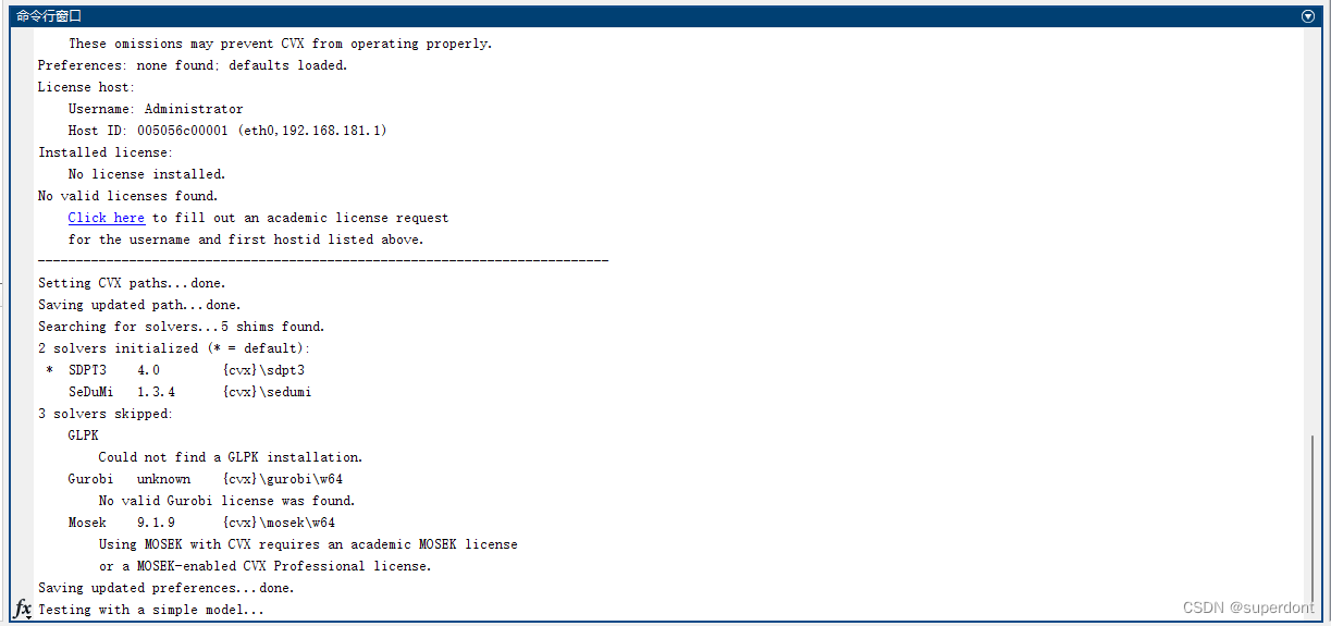
安装过程：

参考文献：
https://zhuanlan.zhihu.com/p/656050116

相关博文

理解并实现OpenCV中的图像平滑技术

OpenCV中的边缘检测技术及实现

OpenCV识别人脸案例实战

入门OpenCV：图像阈值处理

我的图书

下面两本书欢迎大家参考学习。

OpenCV轻松入门

李立宗，OpenCV轻松入门，电子工业出版社，2023
本书基于面向 Python 的 OpenCV(OpenCV for Python)，介绍了图像处理的方方面面。本书以 OpenCV 官方文档的知识脉络为主线，并对细节进行补充和说明。书中不仅介绍了 OpenCV 函数的使用方法，还介绍了函数实现的算法原理。

在介绍 OpenCV 函数的使用方法时，提供了大量的程序示例，并以循序渐进的方式展开。首先，直观地展示函数在易于观察的小数组上的使用方法、处理过程、运行结果，方便读者更深入地理解函数的原理、使用方法、运行机制、处理结果。在此基础上，进一步介绍如何更好地使用函数处理图像。在介绍具体的算法原理时，本书尽量使用通俗易懂的语言和贴近生活的实例来说明问题，避免使用过多复杂抽象的公式。

本书适合计算机视觉领域的初学者阅读，包括在校学生、教师、专业技术人员、图像处理爱好者。
本书第1版出版后，深受广大读者朋友的喜爱，被很多高校选为教材，目前已经累计重印9次。为了更好地方便大家学习，对本书进行了修订。

计算机视觉40例

李立宗，计算机视觉40例，电子工业出版社，2022
近年来，我深耕计算机视觉领域的课程研发工作，在该领域尤其是OpenCV-Python方面积累了一点儿经验。因此，我经常会收到该领域相关知识点的咨询，内容涵盖图像处理的基础知识、OpenCV工具的使用、深度学习的具体应用等多个方面。为了更好地把所积累的知识以图文的形式分享给大家，我将该领域内的知识点进行了系统的整理，编写了本书。希望本书的内容能够对大家在计算机视觉方向的学习有所帮助。
本书以OpenCV-Python（the Python API for OpenCV）为工具，以案例为载体，系统介绍了计算机视觉从入门到深度学习的相关知识点。
本书从计算机视觉基础、经典案例、机器学习、深度学习、人脸识别应用等五个方面对计算机视觉的相关知识点做了全面、系统、深入的介绍。书中共介绍了40余个经典的计算机视觉案例，其中既有字符识别、信息加密、指纹识别、车牌识别、次品检测等计算机视觉的经典案例，也包含图像分类、目标检测、语义分割、实例分割、风格迁移、姿势识别等基于深度学习的计算机视觉案例，还包括表情识别、驾驶员疲劳监测、易容术、识别年龄和性别等针对人脸的应用案例。
在介绍具体的算法原理时，本书尽量使用通俗易懂的语言和贴近生活的示例来说明问题，避免使用复杂抽象的公式来介绍。
本书适合计算机视觉领域的初学者阅读，适于在校学生、教师、专业技术人员、图像处理爱好者使用。

这篇关于MATLAB通过cvx计算L1仿真压缩感知的文章就介绍到这儿，希望我们推荐的文章对编程师们有所帮助！

---