Advanced Lane Detection源码解读（二）

本文主要是介绍Advanced Lane Detection源码解读（二），希望对大家解决编程问题提供一定的参考价值，需要的开发者们随着小编来一起学习吧！

1.2.2 二次曲线拟合 line_fit.py

1. 引入相关的包

import numpy as np
import cv2
import matplotlib.pyplot as plt
import matplotlib.image as mpimg
import pickle
from combined_thresh import combined_thresh
from perspective_transform import perspective_transform

2. 由二值图像进行曲线拟合（首帧）
   

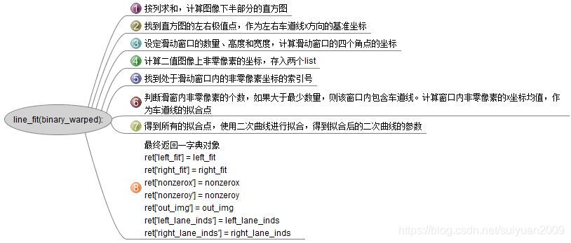
def line_fit(binary_warped):"""Find and fit lane lines"""# Assuming you have created a warped binary image called "binary_warped"# Take a histogram of the bottom half of the image# 求图像下半部分的直方图，np.sum( , axis=0)，# 当axis为0时,是压缩行,即将每一列的元素相加,将矩阵压缩为一行# 当axis为1时,是压缩列,即将每一行的元素相加,将矩阵压缩为一列(这里的一列是为了方便理解说的，实际上，在控制台的输出中，仍然是以一行的形式输出的)histogram = np.sum(binary_warped[binary_warped.shape[0]//2:,:], axis=0)# Create an output image to draw on and visualize the resultout_img = (np.dstack((binary_warped, binary_warped, binary_warped))*255).astype('uint8')# Find the peak of the left and right halves of the histogram# These will be the starting point for the left and right linesmidpoint = np.int(histogram.shape[0]/2)leftx_base = np.argmax(histogram[100:midpoint]) + 100 # 在100:midpoint范围内寻找的直方图的最大值点，将其x坐标存为leftx_base rightx_base = np.argmax(histogram[midpoint:-100]) + midpoint # midpoint:-100范围内寻找的直方图的最大值点，将其x坐标存为rightx_base # Choose the number of sliding windows# 选择图像上滑动窗口的数量nwindows = 9 # Set height of windows# 设置滑动窗口的高度=图像高度/滑窗数量window_height = np.int(binary_warped.shape[0]/nwindows)# Identify the x and y positions of all nonzero pixels in the image# 找到二值图中所有非零像素的坐标。numpy.nonzero()，当调用对象为二维数组时，返回的为长度为2的元组。nonzero = binary_warped.nonzero()nonzeroy = np.array(nonzero[0])nonzerox = np.array(nonzero[1])# Current positions to be updated for each windowleftx_current = leftx_baserightx_current = rightx_base# Set the width of the windows +/- marginmargin = 100# Set minimum number of pixels found to recenter windowminpix = 50# Create empty lists to receive left and right lane pixel indicesleft_lane_inds = []right_lane_inds = []# Step through the windows one by onefor window in range(nwindows):# Identify window boundaries in x and y (and right and left)# 得到滑窗四个角点的坐标win_y_low = binary_warped.shape[0] - (window+1)*window_heightwin_y_high = binary_warped.shape[0] - window*window_heightwin_xleft_low = leftx_current - marginwin_xleft_high = leftx_current + marginwin_xright_low = rightx_current - marginwin_xright_high = rightx_current + margin# Draw the windows on the visualization imagecv2.rectangle(out_img,(win_xleft_low,win_y_low),(win_xleft_high,win_y_high),(0,255,0), 2)cv2.rectangle(out_img,(win_xright_low,win_y_low),(win_xright_high,win_y_high),(0,255,0), 2)# Identify the nonzero pixels in x and y within the window# 挑选出位于滑窗内的非零像素点good_left_inds = ((nonzeroy >= win_y_low) & (nonzeroy < win_y_high) & (nonzerox >= win_xleft_low) & (nonzerox < win_xleft_high)).nonzero()[0]good_right_inds = ((nonzeroy >= win_y_low) & (nonzeroy < win_y_high) & (nonzerox >= win_xright_low) & (nonzerox < win_xright_high)).nonzero()[0]# Append these indices to the listsleft_lane_inds.append(good_left_inds)right_lane_inds.append(good_right_inds)# If you found > minpix pixels, recenter next window on their mean positionif len(good_left_inds) > minpix:leftx_current = np.int(np.mean(nonzerox[good_left_inds]))if len(good_right_inds) > minpix:rightx_current = np.int(np.mean(nonzerox[good_right_inds]))# Concatenate the arrays of indicesleft_lane_inds = np.concatenate(left_lane_inds)right_lane_inds = np.concatenate(right_lane_inds)# Extract left and right line pixel positionsleftx = nonzerox[left_lane_inds]lefty = nonzeroy[left_lane_inds]rightx = nonzerox[right_lane_inds]righty = nonzeroy[right_lane_inds]# Fit a second order polynomial to eachleft_fit = np.polyfit(lefty, leftx, 2)right_fit = np.polyfit(righty, rightx, 2)# Return a dict of relevant variablesret = {}ret['left_fit'] = left_fitret['right_fit'] = right_fitret['nonzerox'] = nonzeroxret['nonzeroy'] = nonzeroyret['out_img'] = out_imgret['left_lane_inds'] = left_lane_indsret['right_lane_inds'] = right_lane_indsreturn ret

4. 由二值图像进行曲线拟合（非首帧）

def tune_fit(binary_warped, left_fit, right_fit):"""Given a previously fit line, quickly try to find the line based on previous lines"""# Assume you now have a new warped binary image# from the next frame of video (also called "binary_warped")# It's now much easier to find line pixels!nonzero = binary_warped.nonzero()nonzeroy = np.array(nonzero[0])nonzerox = np.array(nonzero[1])margin = 100left_lane_inds = ((nonzerox > (left_fit[0]*(nonzeroy**2) + left_fit[1]*nonzeroy + left_fit[2] - margin)) & (nonzerox < (left_fit[0]*(nonzeroy**2) + left_fit[1]*nonzeroy + left_fit[2] + margin)))right_lane_inds = ((nonzerox > (right_fit[0]*(nonzeroy**2) + right_fit[1]*nonzeroy + right_fit[2] - margin)) & (nonzerox < (right_fit[0]*(nonzeroy**2) + right_fit[1]*nonzeroy + right_fit[2] + margin)))# Again, extract left and right line pixel positionsleftx = nonzerox[left_lane_inds]lefty = nonzeroy[left_lane_inds]rightx = nonzerox[right_lane_inds]righty = nonzeroy[right_lane_inds]# If we don't find enough relevant points, return all None (this means error)min_inds = 10if lefty.shape[0] < min_inds or righty.shape[0] < min_inds:return None# Fit a second order polynomial to eachleft_fit = np.polyfit(lefty, leftx, 2)right_fit = np.polyfit(righty, rightx, 2)# Generate x and y values for plottingploty = np.linspace(0, binary_warped.shape[0]-1, binary_warped.shape[0] )left_fitx = left_fit[0]*ploty**2 + left_fit[1]*ploty + left_fit[2]right_fitx = right_fit[0]*ploty**2 + right_fit[1]*ploty + right_fit[2]# Return a dict of relevant variablesret = {}ret['left_fit'] = left_fitret['right_fit'] = right_fitret['nonzerox'] = nonzeroxret['nonzeroy'] = nonzeroyret['left_lane_inds'] = left_lane_indsret['right_lane_inds'] = right_lane_indsreturn ret

5. 可视化1

def viz1(binary_warped, ret, save_file=None):"""Visualize each sliding window location and predicted lane lines, on binary warped imagesave_file is a string representing where to save the image (if None, then just display)"""# Grab variables from ret dictionaryleft_fit = ret['left_fit']right_fit = ret['right_fit']nonzerox = ret['nonzerox']nonzeroy = ret['nonzeroy']out_img = ret['out_img']left_lane_inds = ret['left_lane_inds']right_lane_inds = ret['right_lane_inds']# Generate x and y values for plottingploty = np.linspace(0, binary_warped.shape[0]-1, binary_warped.shape[0] )left_fitx = left_fit[0]*ploty**2 + left_fit[1]*ploty + left_fit[2]right_fitx = right_fit[0]*ploty**2 + right_fit[1]*ploty + right_fit[2]out_img[nonzeroy[left_lane_inds], nonzerox[left_lane_inds]] = [255, 0, 0]out_img[nonzeroy[right_lane_inds], nonzerox[right_lane_inds]] = [0, 0, 255]plt.imshow(out_img)plt.plot(left_fitx, ploty, color='yellow')plt.plot(right_fitx, ploty, color='yellow')plt.xlim(0, 1280)plt.ylim(720, 0)if save_file is None:plt.show()else:plt.savefig(save_file)plt.gcf().clear()

6. 可视化2

def viz2(binary_warped, ret, save_file=None):"""Visualize the predicted lane lines with margin, on binary warped imagesave_file is a string representing where to save the image (if None, then just display)"""# Grab variables from ret dictionaryleft_fit = ret['left_fit']right_fit = ret['right_fit']nonzerox = ret['nonzerox']nonzeroy = ret['nonzeroy']left_lane_inds = ret['left_lane_inds']right_lane_inds = ret['right_lane_inds']# Create an image to draw on and an image to show the selection windowout_img = (np.dstack((binary_warped, binary_warped, binary_warped))*255).astype('uint8')window_img = np.zeros_like(out_img)# Color in left and right line pixelsout_img[nonzeroy[left_lane_inds], nonzerox[left_lane_inds]] = [255, 0, 0]out_img[nonzeroy[right_lane_inds], nonzerox[right_lane_inds]] = [0, 0, 255]# Generate x and y values for plottingploty = np.linspace(0, binary_warped.shape[0]-1, binary_warped.shape[0])left_fitx = left_fit[0]*ploty**2 + left_fit[1]*ploty + left_fit[2]right_fitx = right_fit[0]*ploty**2 + right_fit[1]*ploty + right_fit[2]# Generate a polygon to illustrate the search window area# And recast the x and y points into usable format for cv2.fillPoly()margin = 100  # NOTE: Keep this in sync with *_fit()left_line_window1 = np.array([np.transpose(np.vstack([left_fitx-margin, ploty]))])left_line_window2 = np.array([np.flipud(np.transpose(np.vstack([left_fitx+margin, ploty])))])left_line_pts = np.hstack((left_line_window1, left_line_window2))right_line_window1 = np.array([np.transpose(np.vstack([right_fitx-margin, ploty]))])right_line_window2 = np.array([np.flipud(np.transpose(np.vstack([right_fitx+margin, ploty])))])right_line_pts = np.hstack((right_line_window1, right_line_window2))# Draw the lane onto the warped blank imagecv2.fillPoly(window_img, np.int_([left_line_pts]), (0,255, 0))cv2.fillPoly(window_img, np.int_([right_line_pts]), (0,255, 0))result = cv2.addWeighted(out_img, 1, window_img, 0.3, 0)plt.imshow(result)plt.plot(left_fitx, ploty, color='yellow')plt.plot(right_fitx, ploty, color='yellow')plt.xlim(0, 1280)plt.ylim(720, 0)if save_file is None:plt.show()else:plt.savefig(save_file)plt.gcf().clear()

7. 计算曲线

def calc_curve(left_lane_inds, right_lane_inds, nonzerox, nonzeroy):"""Calculate radius of curvature in meters"""y_eval = 719  # 720p video/image, so last (lowest on screen) y index is 719# Define conversions in x and y from pixels space to metersym_per_pix = 30/720 # meters per pixel in y dimensionxm_per_pix = 3.7/700 # meters per pixel in x dimension# Extract left and right line pixel positionsleftx = nonzerox[left_lane_inds]lefty = nonzeroy[left_lane_inds]rightx = nonzerox[right_lane_inds]righty = nonzeroy[right_lane_inds]# Fit new polynomials to x,y in world spaceleft_fit_cr = np.polyfit(lefty*ym_per_pix, leftx*xm_per_pix, 2)right_fit_cr = np.polyfit(righty*ym_per_pix, rightx*xm_per_pix, 2)# Calculate the new radii of curvatureleft_curverad = ((1 + (2*left_fit_cr[0]*y_eval*ym_per_pix + left_fit_cr[1])**2)**1.5) / np.absolute(2*left_fit_cr[0])right_curverad = ((1 + (2*right_fit_cr[0]*y_eval*ym_per_pix + right_fit_cr[1])**2)**1.5) / np.absolute(2*right_fit_cr[0])# Now our radius of curvature is in metersreturn left_curverad, right_curverad

8. 计算车辆偏移道路中心

def calc_vehicle_offset(undist, left_fit, right_fit):"""Calculate vehicle offset from lane center, in meters"""# Calculate vehicle center offset in pixelsbottom_y = undist.shape[0] - 1bottom_x_left = left_fit[0]*(bottom_y**2) + left_fit[1]*bottom_y + left_fit[2]bottom_x_right = right_fit[0]*(bottom_y**2) + right_fit[1]*bottom_y + right_fit[2]vehicle_offset = undist.shape[1]/2 - (bottom_x_left + bottom_x_right)/2# Convert pixel offset to metersxm_per_pix = 3.7/700 # meters per pixel in x dimensionvehicle_offset *= xm_per_pixreturn vehicle_offset

9. 最终显示

def final_viz(undist, left_fit, right_fit, m_inv, left_curve, right_curve, vehicle_offset):"""Final lane line prediction visualized and overlayed on top of original image"""# Generate x and y values for plottingploty = np.linspace(0, undist.shape[0]-1, undist.shape[0])left_fitx = left_fit[0]*ploty**2 + left_fit[1]*ploty + left_fit[2]right_fitx = right_fit[0]*ploty**2 + right_fit[1]*ploty + right_fit[2]# Create an image to draw the lines on#warp_zero = np.zeros_like(warped).astype(np.uint8)#color_warp = np.dstack((warp_zero, warp_zero, warp_zero))color_warp = np.zeros((720, 1280, 3), dtype='uint8')  # NOTE: Hard-coded image dimensions# Recast the x and y points into usable format for cv2.fillPoly()pts_left = np.array([np.transpose(np.vstack([left_fitx, ploty]))])pts_right = np.array([np.flipud(np.transpose(np.vstack([right_fitx, ploty])))])pts = np.hstack((pts_left, pts_right))# Draw the lane onto the warped blank imagecv2.fillPoly(color_warp, np.int_([pts]), (0,255, 0))# Warp the blank back to original image space using inverse perspective matrix (Minv)newwarp = cv2.warpPerspective(color_warp, m_inv, (undist.shape[1], undist.shape[0]))# Combine the result with the original imageresult = cv2.addWeighted(undist, 1, newwarp, 0.3, 0)# Annotate lane curvature values and vehicle offset from centeravg_curve = (left_curve + right_curve)/2label_str = 'Radius of curvature: %.1f m' % avg_curveresult = cv2.putText(result, label_str, (30,40), 0, 1, (0,0,0), 2, cv2.LINE_AA)label_str = 'Vehicle offset from lane center: %.1f m' % vehicle_offsetresult = cv2.putText(result, label_str, (30,70), 0, 1, (0,0,0), 2, cv2.LINE_AA)return result

这篇关于Advanced Lane Detection源码解读（二）的文章就介绍到这儿，希望我们推荐的文章对编程师们有所帮助！

---