【实验笔记】Python3+OpenCV读表盘示数

源码来自于GitHub，https://github.com/intel-iot-devkit/python-cv-samples，源码是Python2，在这里修改为Python3。并做一些分析记录

将GitHub上的项目下载到本地，这里存放在/home/dingzhihui/Downloads目录下,解压，通过PyCharm打开analog_gauge_reader.py文件
首先记录一下运行成功需要修改的部分：
1.读取图片的路径，在这里将图片路径换为绝对路径，便可读取

修改前：

img = cv2.imread('gauge-%s.%s' %(gauge_number, file_type))

修改后：

img = cv2.imread('/home/dingzhihui/Downloads/python-cv-samples-master/examples/analog-gauge-reader/images/gauge-%s.%s' %(gauge_number, file_type))

1.cv2.imread（）返回值为NONE

执行pip install --upgrade opencv-python，成功后重新打开python console验证，imread jpg通过，返回的img为正常的MN3数据；至此解决此错误。
修改图片路径：

img = cv2.imread('/usr/apps/python-cv-samples-master/examples/analog-gauge-reader/images/gauge-1.jpg',cv2.IMREAD_UNCHANGED)

2.python3将raw_input和input进行了整合，只有input

gray2 = cv2.cvtColor(img, cv2.COLOR_BGR2GRAY)

'''  
Copyright (c) 2017 Intel Corporation.
Licensed under the MIT license. See LICENSE file in the project root for full license information.
'''import cv2
import numpy as np
#import paho.mqtt.client as mqtt
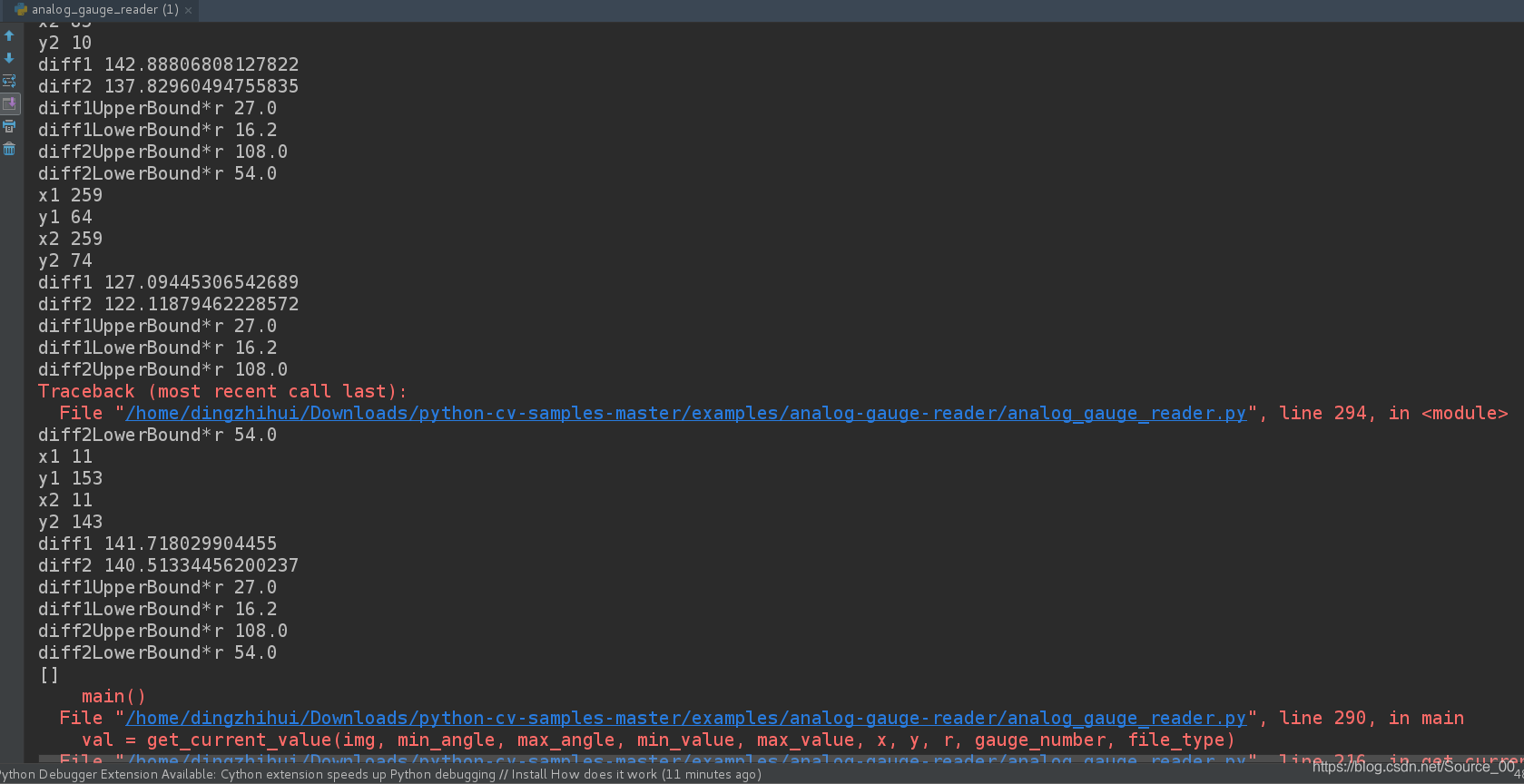
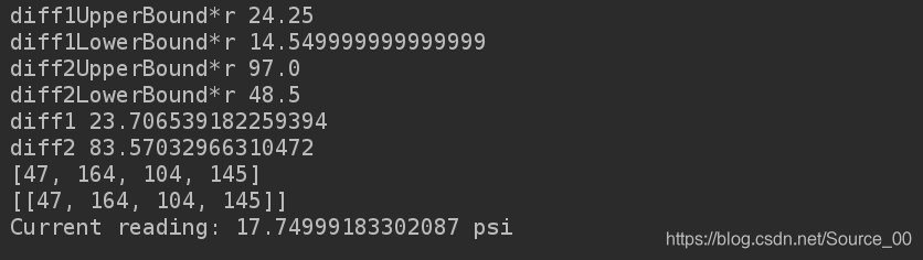
import timedef avg_circles(circles, b):avg_x=0avg_y=0avg_r=0for i in range(b):#optional - average for multiple circles (can happen when a gauge is at a slight angle)avg_x = avg_x + circles[0][i][0]avg_y = avg_y + circles[0][i][1]avg_r = avg_r + circles[0][i][2]avg_x = int(avg_x/(b))avg_y = int(avg_y/(b))avg_r = int(avg_r/(b))return avg_x, avg_y, avg_rdef dist_2_pts(x1, y1, x2, y2):#print np.sqrt((x2-x1)^2+(y2-y1)^2)return np.sqrt((x2 - x1)**2 + (y2 - y1)**2)def calibrate_gauge(gauge_number, file_type):'''This function should be run using a test image in order to calibrate the range available to the dial as well as theunits.  It works by first finding the center point and radius of the gauge.  Then it draws lines at hard coded intervals(separation) in degrees.  It then prompts the user to enter position in degrees of the lowest possible value of the gauge,as well as the starting value (which is probably zero in most cases but it won't assume that).  It will then ask for theposition in degrees of the largest possible value of the gauge. Finally, it will ask for the units.  This assumes thatthe gauge is linear (as most probably are).It will return the min value with angle in degrees (as a tuple), the max value with angle in degree45s (as a tuple),and the units (as a string).这个函数用测试图片来校准刻度盘和刻度盘可用的范围单位。需要之前所得的中心点以及半径。然后绘制出刻度。需要输入表盘读数最小角度，最大角度,最小值，最大值，以及单位(min_angle,max_angle,min_value,max_value,units)        '''img = cv2.imread('/home/dingzhihui/Downloads/python-cv-samples-master/examples/analog-gauge-reader/images/gauge-%s.%s' %(gauge_number, file_type))print(img)height, width = img.shape[:2]#将图片转为灰度图片gray = cv2.cvtColor(img, cv2.COLOR_BGR2GRAY)  #convert to gray#gray = cv2.GaussianBlur(gray, (5, 5), 0)# gray = cv2.medianBlur(gray, 5)#for testing, output gray image#cv2.imwrite('gauge-%s-bw.%s' %(gauge_number, file_type),gray)#detect circles#restricting the search from 35-48% of the possible radii gives fairly good results across different samples.  Remember that#these are pixel values which correspond to the possible radii search range.#霍夫圆环检测#image:8位，单通道图像#method：定义检测图像中圆的方法。目前唯一实现的方法cv2.HOUGH_GRADIENT。#dp：累加器分辨率与图像分辨率的反比。dp获取越大，累加器数组越小。#minDist：检测到的圆的中心，（x,y）坐标之间的最小距离。如果minDist太小，则可能导致检测到多个相邻的圆。如果minDist太大，则可能导致很多圆检测不到。#param1：用于处理边缘检测的梯度值方法。#param2：cv2.HOUGH_GRADIENT方法的累加器阈值。阈值越小，检测到的圈子越多。#minRadius：半径的最小大小（以像素为单位）。#maxRadius：半径的最大大小（以像素为单位）。circles = cv2.HoughCircles(gray, cv2.HOUGH_GRADIENT, 1, 20, np.array([]), 100, 50, int(height*0.35), int(height*0.48))# average found circles, found it to be more accurate than trying to tune HoughCircles parameters to get just the right onea, b, c = circles.shape#获取圆的坐标x,y和半径rx,y,r = avg_circles(circles, b)#draw center and circlecv2.circle(img, (x, y), r, (0, 0, 255), 3, cv2.LINE_AA)  # draw circlecv2.circle(img, (x, y), 2, (0, 255, 0), 3, cv2.LINE_AA)  # draw center of circle#for testing, output circles on image#cv2.imwrite('gauge-%s-circles.%s' % (gauge_number, file_type), img)#for calibration, plot lines from center going out at every 10 degrees and add marker#for i from 0 to 36 (every 10 deg)'''goes through the motion of a circle and sets x and y values based on the set separation spacing.  Also adds text to eachline.  These lines and text labels serve as the reference point for the user to enterNOTE: by default this approach sets 0/360 to be the +x axis (if the image has a cartesian grid in the middle), the addition(i+9) in the text offset rotates the labels by 90 degrees so 0/360 is at the bottom (-y in cartesian).  So this assumes thegauge is aligned in the image, but it can be adjusted by changing the value of 9 to something else.根据画出的刻度值，给定x，y的值，并在此位置添加文本信息。这些刻度和文本标签用作用户输入的参考点'''separation = 10.0 #in degreesinterval = int(360 / separation)p1 = np.zeros((interval,2))  #set empty arraysp2 = np.zeros((interval,2))p_text = np.zeros((interval,2))for i in range(0,interval):for j in range(0,2):if (j%2==0):p1[i][j] = x + 0.9 * r * np.cos(separation * i * 3.14 / 180) #point for lineselse:p1[i][j] = y + 0.9 * r * np.sin(separation * i * 3.14 / 180)text_offset_x = 10text_offset_y = 5for i in range(0, interval):for j in range(0, 2):if (j % 2 == 0):p2[i][j] = x + r * np.cos(separation * i * 3.14 / 180)p_text[i][j] = x - text_offset_x + 1.2 * r * np.cos((separation) * (i+9) * 3.14 / 180) #point for text labels, i+9 rotates the labels by 90 degreeselse:p2[i][j] = y + r * np.sin(separation * i * 3.14 / 180)p_text[i][j] = y + text_offset_y + 1.2* r * np.sin((separation) * (i+9) * 3.14 / 180)  # point for text labels, i+9 rotates the labels by 90 degrees#add the lines and labels to the imagefor i in range(0,interval):cv2.line(img, (int(p1[i][0]), int(p1[i][1])), (int(p2[i][0]), int(p2[i][1])),(0, 255, 0), 2)cv2.putText(img, '%s' %(int(i*separation)), (int(p_text[i][0]), int(p_text[i][1])), cv2.FONT_HERSHEY_SIMPLEX, 0.3,(0,0,0),1,cv2.LINE_AA)cv2.imwrite('gauge-%s-calibration.%s' % (gauge_number, file_type), img)#get user input on min, max, values, and unitsprint ('gauge number: %s' %gauge_number)min_angle = input('Min angle (lowest possible angle of dial) - in degrees: ') #the lowest possible anglemax_angle = input('Max angle (highest possible angle) - in degrees: ') #highest possible anglemin_value = input('Min value: ') #usually zeromax_value = input('Max value: ') #maximum reading of the gaugeunits = input('Enter units: ')#for testing purposes: hardcode and comment out raw_inputs above# min_angle = 45# max_angle = 320# min_value = 0# max_value = 200# units = "PSI"return min_angle, max_angle, min_value, max_value, units, x, y, rdef get_current_value(img, min_angle, max_angle, min_value, max_value, x, y, r, gauge_number, file_type):#for testing purposes#img = cv2.imread('gauge-%s.%s' % (gauge_number, file_type))gray2 = cv2.cvtColor(img, cv2.COLOR_BGR2GRAY)# Set threshold and maxValuethresh = 175maxValue = 255# for testing purposes, found cv2.THRESH_BINARY_INV to perform the best# th, dst1 = cv2.threshold(gray2, thresh, maxValue, cv2.THRESH_BINARY);# th, dst2 = cv2.threshold(gray2, thresh, maxValue, cv2.THRESH_BINARY_INV);# th, dst3 = cv2.threshold(gray2, thresh, maxValue, cv2.THRESH_TRUNC);# th, dst4 = cv2.threshold(gray2, thresh, maxValue, cv2.THRESH_TOZERO);# th, dst5 = cv2.threshold(gray2, thresh, maxValue, cv2.THRESH_TOZERO_INV);# cv2.imwrite('gauge-%s-dst1.%s' % (gauge_number, file_type), dst1)# cv2.imwrite('gauge-%s-dst2.%s' % (gauge_number, file_type), dst2)# cv2.imwrite('gauge-%s-dst3.%s' % (gauge_number, file_type), dst3)# cv2.imwrite('gauge-%s-dst4.%s' % (gauge_number, file_type), dst4)# cv2.imwrite('gauge-%s-dst5.%s' % (gauge_number, file_type), dst5)# apply thresholding which helps for finding linesth, dst2 = cv2.threshold(gray2, thresh, maxValue, cv2.THRESH_BINARY_INV);# found Hough Lines generally performs better without Canny / blurring, though there were a couple exceptions where it would only work with Canny / blurring#dst2 = cv2.medianBlur(dst2, 5)#dst2 = cv2.Canny(dst2, 50, 150)#dst2 = cv2.GaussianBlur(dst2, (5, 5), 0)# for testing, show image after thresholdingcv2.imwrite('gauge-%s-tempdst2.%s' % (gauge_number, file_type), dst2)# find linesminLineLength = 10maxLineGap = 0lines = cv2.HoughLinesP(image=dst2, rho=3, theta=np.pi / 180, threshold=100,minLineLength=minLineLength, maxLineGap=0)  # rho is set to 3 to detect more lines, easier to get more then filter them out later#for testing purposes, show all found lines# for i in range(0, len(lines)):#   for x1, y1, x2, y2 in lines[i]:#      cv2.line(img, (x1, y1), (x2, y2), (0, 255, 0), 2)#      cv2.imwrite('gauge-%s-lines-test.%s' %(gauge_number, file_type), img)# remove all lines outside a given radiusprint('lines',lines)final_line_list = []#print "radius: %s" %rdiff1LowerBound = 0.15 #diff1LowerBound and diff1UpperBound determine how close the line should be from the centerdiff1UpperBound = 0.25diff2LowerBound = 0.5 #diff2LowerBound and diff2UpperBound determine how close the other point of the line should be to the outside of the gaugediff2UpperBound = 1.0for i in range(0, len(lines)):for x1, y1, x2, y2 in lines[i]:#print('x1',x1)#print('y1',y1)#print('x2',x2)#print('y2',y2)diff1 = dist_2_pts(x, y, x1, y1)  # x, y is center of circle#print('diff1',diff1)diff2 = dist_2_pts(x, y, x2, y2)  # x, y is center of circle#print('diff2', diff2)#set diff1 to be the smaller (closest to the center) of the two), makes the math easierif (diff1 > diff2):temp = diff1diff1 = diff2diff2 = temp# check if line is within an acceptable range#print('diff1UpperBound*r',diff1UpperBound*r)#print('diff1LowerBound*r', diff1LowerBound*r)#print('diff2UpperBound*r', diff2UpperBound*r)#print('diff2LowerBound*r', diff2LowerBound*r)if (((diff1<diff1UpperBound*r) and (diff1>diff1LowerBound*r) and (diff2<diff2UpperBound*r)) and (diff2>diff2LowerBound*r)):print('aaaaaaaaaaaaaaaaaaaaaaaaaaaaaaaaaaaaaaaaaaaaaaaaaaaaaaaaaaaaaaaaaaaaaaaaaaaaaaaaaaaaa')print('diff1UpperBound*r',diff1UpperBound*r)print('diff1LowerBound*r', diff1LowerBound*r)print('diff2UpperBound*r', diff2UpperBound*r)print('diff2LowerBound*r', diff2LowerBound*r)print('diff1', diff1)print('diff2', diff2)line_length = dist_2_pts(x1, y1, x2, y2)# add to final listprint([x1, y1, x2, y2])final_line_list.append([x1, y1, x2, y2])#testing only, show all lines after filtering# for i in range(0,len(final_line_list)):#     x1 = final_line_list[i][0]#     y1 = final_line_list[i][1]#     x2 = final_line_list[i][2]#     y2 = final_line_list[i][3]#     cv2.line(img, (x1, y1), (x2, y2), (0, 255, 0), 2)# assumes the first line is the best oneprint(final_line_list)x1 = final_line_list[0][0]y1 = final_line_list[0][1]x2 = final_line_list[0][2]y2 = final_line_list[0][3]cv2.line(img, (x1, y1), (x2, y2), (0, 255, 0), 2)#for testing purposes, show the line overlayed on the original image#cv2.imwrite('gauge-1-test.jpg', img)cv2.imwrite('gauge-%s-lines-2.%s' % (gauge_number, file_type), img)#find the farthest point from the center to be what is used to determine the angledist_pt_0 = dist_2_pts(x, y, x1, y1)dist_pt_1 = dist_2_pts(x, y, x2, y2)if (dist_pt_0 > dist_pt_1):x_angle = x1 - xy_angle = y - y1else:x_angle = x2 - xy_angle = y - y2# take the arc tan of y/x to find the angleres = np.arctan(np.divide(float(y_angle), float(x_angle)))#np.rad2deg(res) #coverts to degrees# print x_angle# print y_angle# print res# print np.rad2deg(res)#these were determined by trial and errorres = np.rad2deg(res)if x_angle > 0 and y_angle > 0:  #in quadrant Ifinal_angle = 270 - resif x_angle < 0 and y_angle > 0:  #in quadrant IIfinal_angle = 90 - resif x_angle < 0 and y_angle < 0:  #in quadrant IIIfinal_angle = 90 - resif x_angle > 0 and y_angle < 0:  #in quadrant IVfinal_angle = 270 - res#print final_angleold_min = float(min_angle)old_max = float(max_angle)new_min = float(min_value)new_max = float(max_value)old_value = final_angleold_range = (old_max - old_min)new_range = (new_max - new_min)new_value = (((old_value - old_min) * new_range) / old_range) + new_minreturn new_valuedef main():gauge_number = 1file_type='jpg'# name the calibration image of your gauge 'gauge-#.jpg', for example 'gauge-5.jpg'.  It's written this way so you can easily try multiple imagesmin_angle, max_angle, min_value, max_value, units, x, y, r = calibrate_gauge(gauge_number, file_type)print('min_angle=',min_angle)print('max_angle=',max_angle)print('min_value=', min_value)print('max_value=', max_value)print('units=', units)print('x=', x)print('y=', y)print('r=', r)#feed an image (or frame) to get the current value, based on the calibration, by default uses same image as calibrationimg = cv2.imread('/home/dingzhihui/Downloads/python-cv-samples-master/examples/analog-gauge-reader/images/gauge-%s.%s' % (gauge_number, file_type))print()val = get_current_value(img, min_angle, max_angle, min_value, max_value, x, y, r, gauge_number, file_type)print("Current reading: %s %s" %(val, units))if __name__=='__main__':main()