RIS 辅助无线网络：基于模型、启发式和机器学习の优化方法

本文主要是介绍RIS 辅助无线网络：基于模型、启发式和机器学习の优化方法，希望对大家解决编程问题提供一定的参考价值，需要的开发者们随着小编来一起学习吧！

A Survey on Model-based, Heuristic, and Machine
Learning Optimization Approaches in RIS-aided
Wireless Networks阅读笔记

abstract

可重构智能表面（RIS）作为设想的 6G 网络的关键推动者受到了广泛关注，其目的是在低能耗和低硬件成本的情况下提高网络容量、覆盖范围、效率和安全性。然而，**将 RIS 集成到现有基础设施中会大大增加网络管理的复杂性，尤其是控制大量 RIS 元素时。**为了充分发挥 RIS 的潜力，有效的优化方法非常重要。这项工作对 RISaided 无线通信的优化技术进行了全面的调查，包括基于模型、启发式和机器学习 (ML) 算法。特别是，我们首先总结了文献中具有不同目标和约束的问题表述，例如总速率最大化、功率最小化和不完善的信道状态信息约束。然后，我们介绍文献中使用的基于模型的算法，例如交替优化、主最小化方法和逐次凸逼近。接下来，讨论启发式优化，它应用启发式规则来获得低复杂度的解决方案。此外，我们还展示了针对 RIS 的最先进的 ML 算法和应用，即监督和无监督学习、强化学习、联邦学习、图学习、迁移学习和基于分层学习的方法。基于模型、启发式和机器学习方法在稳定性、鲁棒性、最优性等方面进行了比较，提供了对这些技术的系统理解。最后，我们重点介绍 RISaided 面向 6G 网络的应用并确定未来的挑战。

integrating RISs into the
existing infrastructure greatly increases the network management
complexity, especially for controlling a significant number of RIS
elements.

introduction

在5G进入商用阶段的同时，研究界也开始了对未来6G网络的探索。与前几代网络相比，6G 网络预计将提出更严格的性能要求，即虚拟现实的太比特每秒 (Tbps) 数据速率、超过 107 个/km2 的连接密度以及显着低于 5G 网络的延迟[1]。无线网络演进的主要障碍之一是具有反射、衍射和散射的不可控无线电环境。最近，可重构智能表面（RIS）已成为增强无线信号传播的一种有前途的技术[2]。特别是，RIS 的核心特征是通过智能配置大量小元件来操纵信号传播路径。每个 RIS 元件都可以独立调整入射信号的相位，从而创建智能无线电环境 [3]。 RIS 不仅在技术上具有吸引力，而且需要低能耗和硬件成本，使该技术成为提高实际部署频谱效率的有前景的技术。鉴于这些优势，RIS 可以与其他新兴技术相结合，包括多输入多输出 (MIMO)、毫米波 (mmWave) 通信、无人机 (UAV) 网络、非正交多址 (NOMA)、车辆万物互联 (V2X) 网络等 [4]、[5]。许多现有的研究和实施已经证明了 RIS 提高网络容量、覆盖范围、能源效率和安全性的能力。

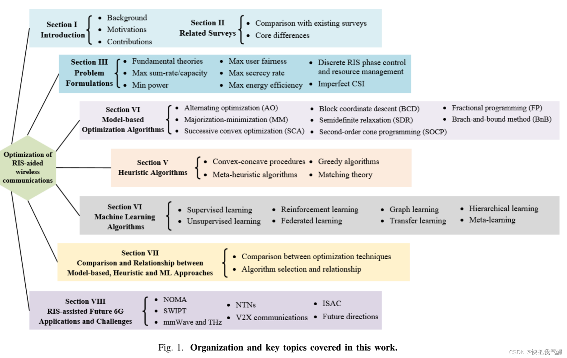
尽管有潜力，但将 RIS 集成到无线网络中将显着增加网络管理的复杂性 [6]。例如，每个 RIS 元件都需要独立的相移配置，从而为优化算法提供巨大的解空间。当共同涉及其他控制变量时，例如波束成形、频谱分配、NOMA 解码顺序或无人机轨迹设计，RIS 配置会更加复杂。因此，先进的优化技术对于处理此类复杂性并充分利用 RIS 至关重要。出于优化技术重要性的推动，这项工作全面概述了 RIS 辅助无线通信的优化技术，包括基于模型、启发式和机器学习 (ML) 方法。有几项调查致力于 RIS 的理论、设计、分析和应用 [7]-[12]。然而，这项工作与现有的调查和教程不同，它系统地总结和分析了 RIS 辅助无线网络的优化技术，提供详细的比较，并包括更多最先进的 ML 技术。具体来说，如图1所示，我们重点关注以下几个方面：

1 问题表述：我们首先介绍RIS技术的基本理论，然后概述RIS辅助无线网络优化的问题表述，包括总速率/容量的最大化、能源效率、用户公平性和保密率，以及最大限度地减少功耗。此外，我们还考虑离散 RIS 相移和资源管理问题，其中包括整数控制变量以及具有不同误差模型约束的不完美通道状态信息 (CSI)。

2 基于模型的方法：在这项工作中，基于模型的方法是指依赖于充分了解所定义问题的特定优化模型的算法。基于模型的算法通常对问题表述的属性和形式有很高的要求，例如凸性、连续性和可微性。我们包括以下基于模型的算法，用于优化 RIS 辅助无线网络：交替优化 (AO)、多数化最小化 (MM) 方法、连续凸优化 (SCA)、块坐标下降 (BCD)、半定松弛 (SDR)、二次优化-阶锥规划（SOCP）、分数规划（FP）和分支定界（BnB）。

3 启发式算法：这些算法应用启发式规则来解决问题。它们通过牺牲最优性和准确性来获得低复杂性和快速的解决方案，为传统的基于模型的方法提供了更有效的替代方案。启发式算法可用于解决 NP 难题或作为其他算法的基线和补充。在本次调查中，我们回顾了用于优化 RIS 辅助无线网络的凸凹过程 (CCP) 算法、元启发式算法、贪婪算法和匹配理论。

4 ML 算法：ML 算法被认为是无线网络优化的有前途的解决方案[16]。机器学习技术不需要完全了解所定义的问题，它们可以从数据中学习或与环境交互来发现隐藏的模式。我们提出了用于优化 RIS 辅助无线网络的最先进的 ML 技术，包括监督和无监督学习、强化学习 (RL)、联邦学习 (FL)、图学习、迁移学习、分层学习和元学习。学习。我们对 RIS 的算法特征和应用进行深入分析，即用于 RIS 相移优化的神经网络数据集获取，以及用于数据速率最大化的无监督神经网络的损失函数定义。此外，我们还比较了基于模型的方法、启发式方法和机器学习方法的最优性、鲁棒性、稳定性等。

5 6G 网络的应用和挑战：我们概述了针对设想的 6G 网络的 RIS 辅助应用，包括 NOMA、同步无线信息和电力传输 (SWIPT)、毫米波和太赫兹通信、非地面网络 (NTN)、V2X 通信和集成传感和通信（ISAC）。此外，我们还确定了 RIS 控制和优化的研究挑战。

总之，这项工作的主要贡献是我们系统地调查了 RISaided 无线网络的优化技术，范围从问题表述到各种方法的特征和应用。我们的工作旨在成为研究人员优化 RISaided 无线网络的路线图。这项工作的其余部分安排如下。第二节回顾了相关工作，而第三节提出了问题的表述。第四节、第五节和第六节分别介绍了基于模型的、启发式的和机器学习优化方法，我们在第七节中对这三种方法进行了比较。第八节包括针对 6G 网络的 RIS 辅助应用并确定了未来的挑战。最后，第九部分总结了本次调查。

相关研究

与RISs相关的研究方向有很多，包括信道建模和估计、信号处理、性能分析、无源波束形成和硬件设计。这项工作的重点是优化技术，由于其至关重要的，表一比较这项工作与现有的调查方面的控制和optimizationrelated的贡献。

表I显示了大多数现有的工作集中在基于模型的方法，包括AO，MM，SCA和SDR。主要原因是这些技术已经被广泛应用，例如，利用自适应光学实现主被动波束的解耦，利用MM和SCA实现非凸目标的近似。启发式算法通常被认为是低复杂度的替代和补充。例如，贪婪算法被用于逐元件RIS相移控制，并且匹配理论被应用于资源分配。然而，尽管它们的重要性，启发式方法被省略在许多现有的调查。同时，ML算法已被广泛应用于无线网络管理，但现有的研究局限于监督学习和RL。此外，一些新出现的技术，如图学习和层次学习，在现有的调查中没有提到。

更具体地说，在许多现有的研究[7]-[10]中，通过介绍文献中使用的算法标题来非常简要地讨论优化技术，但不包括动机和算法特征。Alghamdi等人概述了RIS的优化和性能分析技术，但它在分析问题公式方面受到限制[12]。在[13]中，Faisal和Choi专门研究了用于RIS辅助无线网络的ML方法，但不包括基于模型的方法和启发式方法。此外，一些最先进的ML技术，包括图学习和分层学习，也没有包括在[13]中。相比之下，[11]中介绍了用于RIS信号处理的多种基于模型的方法，但未涵盖许多启发式和ML技术。Liu等人提出了用于RIS辅助无线网络的RIS波束成形、资源管理和ML，但仅详细介绍了RL [14]。监督学习，无监督学习和FL在[14]中进行了简要讨论，而更新的技术，如图学习，迁移学习和分层学习，则没有涉及。在[15]中，Zheng等人调查了不完美/统计/混合CSI下的信道估计和实际RIS控制，但未包括一些优化技术。

这项工作与现有研究的不同之处在于以下方面：

1 控制和优化已经包括在许多调查中，但这项工作是第一次系统地调查的RIS辅助无线网络的优化技术，从问题的配方，步骤，功能，优点和困难的近20种技术。

2 我们提出了深入的分析，将这些优化技术应用到RISs。例如，深度神经网络（DNN）和深度强化学习（DRL）被包括在许多现有的调查中，但一些重要的问题没有讨论，即，数据集采集，用于在RIS辅助环境中进行神经网络训练，并为RL启用的RIS控制定制状态、动作和奖励函数定义。这些问题的答案对于充分利用RISs至关重要。

3 最后，我们提出了最先进的ML技术，用于优化RIS辅助的无线网络，例如，图学习、迁移学习和分层学习，据我们所知，这些都没有包括在现有的调查中。这些新技术可能会带来新的研究方向。

总而言之，本调查回答了以下问题：优化RIS辅助无线网络的最新技术是什么？它们如何涵盖彼此的不同方面？

BACKGROUND AND PROBLEM FORMULATIONS FOR OPTIMIZING RIS-AIDED WIRELESS NETWORKS

A 优化RIS-AIDED无线网络的背景和问题公式

RIS操作原则：

RIS控制：

RIS部署

B 总速率/容量最大化

C 功率最小化

D 能源效率最大化

E 用户公平最大化

F 最大化保密速率

G 带约束的优化：离散RIS相移和资源分配问题

H 非理想CSI的优化约束

---

RIS 辅助无线网络基于模型的优化算法

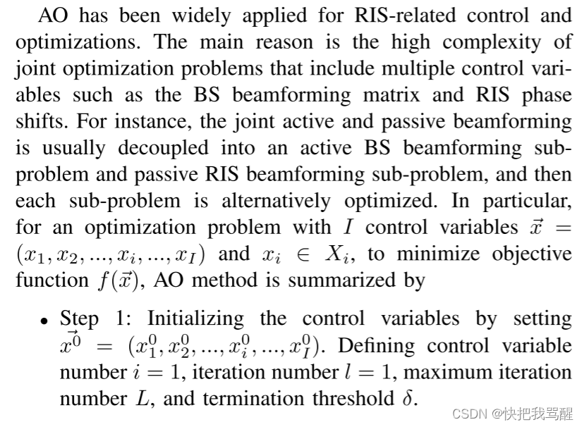
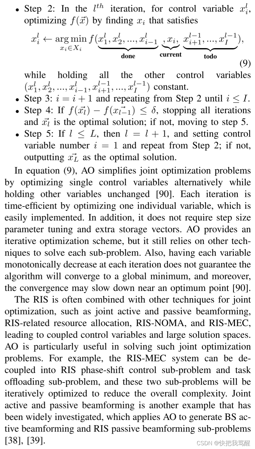
Alternating Optimization(AO)

Block Coordinate Descent(BCD)

坐标下降是解决大规模优化问题的一种非常有用的方法，BCD 被认为是提高计算效率的通用版本。与AO相比，BCD算法中的每个块可以包含多个控制变量，从而能够动态地生成、选择和更新块。因此，BCD方法比AO方法更适合同时优化大量控制变量，已广泛应用于RIS相关的优化问题。

BCD method sequentially minimizes the objective function $F(\vec{x})$ in each block $x_i$ while the other blocks are held fixed. Specifically, it minimizes $x_i^l\leftarrow \underset{x_i\in \mathcal{X}}{\mathrm{argmin}}\left(f\left(x_i\right)+f_i\left(x_i\right)\right)$ while holding other blocks $x_1,x_2,\dots ,x_{i-1},x_{i+1},\dots x_I$ fixed. However, it is worth noting that each block consists of multiple control variables, and the block selection and updating method will affect the BCD performance. An ideal block selection method is expected to maximize the improvement by choosing the blocks that decrease $F(\vec{x})$ by the largest amount [91]. On the other hand, there are many alternatives for the block updating method such as block proximal updating

BCD 方法依次最小化每个块 $x_i$ 中的目标函数 $F(\vec{x})$，而其他块保持固定。具体来说，它最小化 $x_i^l\leftarrow \underset{x_i\in \mathcal{X}}{\mathrm{argmin}}\left(f\left(x_i\right)+f_i\left(x_i\right)\right)$，同时保持其他块 $x_1,x_2,\dots ,x_{i-1},x_{i+1},\dots x_I$ 固定。但值得注意的是，每个块由多个控制变量组成，块的选择和更新方法会影响BCD性能。理想的块选择方法预计通过选择使 $F(\vec{x})$减少最大量的块来最大化改进[91]。另一方面，块更新方法有很多替代方法，例如块近端更新

$$x_i^l\leftarrow \underset{x_i\in \mathcal{X}}{\mathrm{argmin}}\left(f\left(x_i\right)+f_i\left(x_i\right)+\frac{L_i^{l-1}}{2}{\Vert x_i-x_i^{l-1}\Vert }^2\right),\text{\hspace{1em}(10)}$$

where $L_i^{l-1}>0$ . Equation (10) is more stable than conventional BCD by including $\frac{L_i^{l-1}}{2}{\Vert x_i-x_i^{l-1}\Vert }^2$ . The BCD algorithm is easily deployed with low memory requirements and iteration costs, allowing parallel or distributed implementations. But the block selection may affect the algorithm performance, and block updating is difficult in some cases.

Similar to $\mathrm{AO}$, $\mathrm{BCD}$ is considered as an iteration-based scheme to reduce problem-solving complexity. BCD has been applied to sum-rate maximization [21], [25], [27], user fairness maximization [37], and power minimization [48]. As an example, a two-block BCD is used to maximize the sum-rate in [27], in which the first block is for BS active beamforming and the second is for RIS passive beamforming, then these blocks are iteratively optimized.

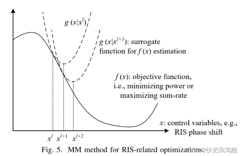
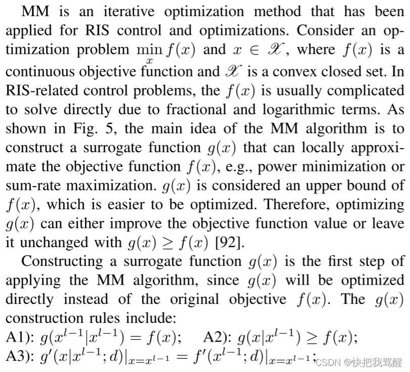
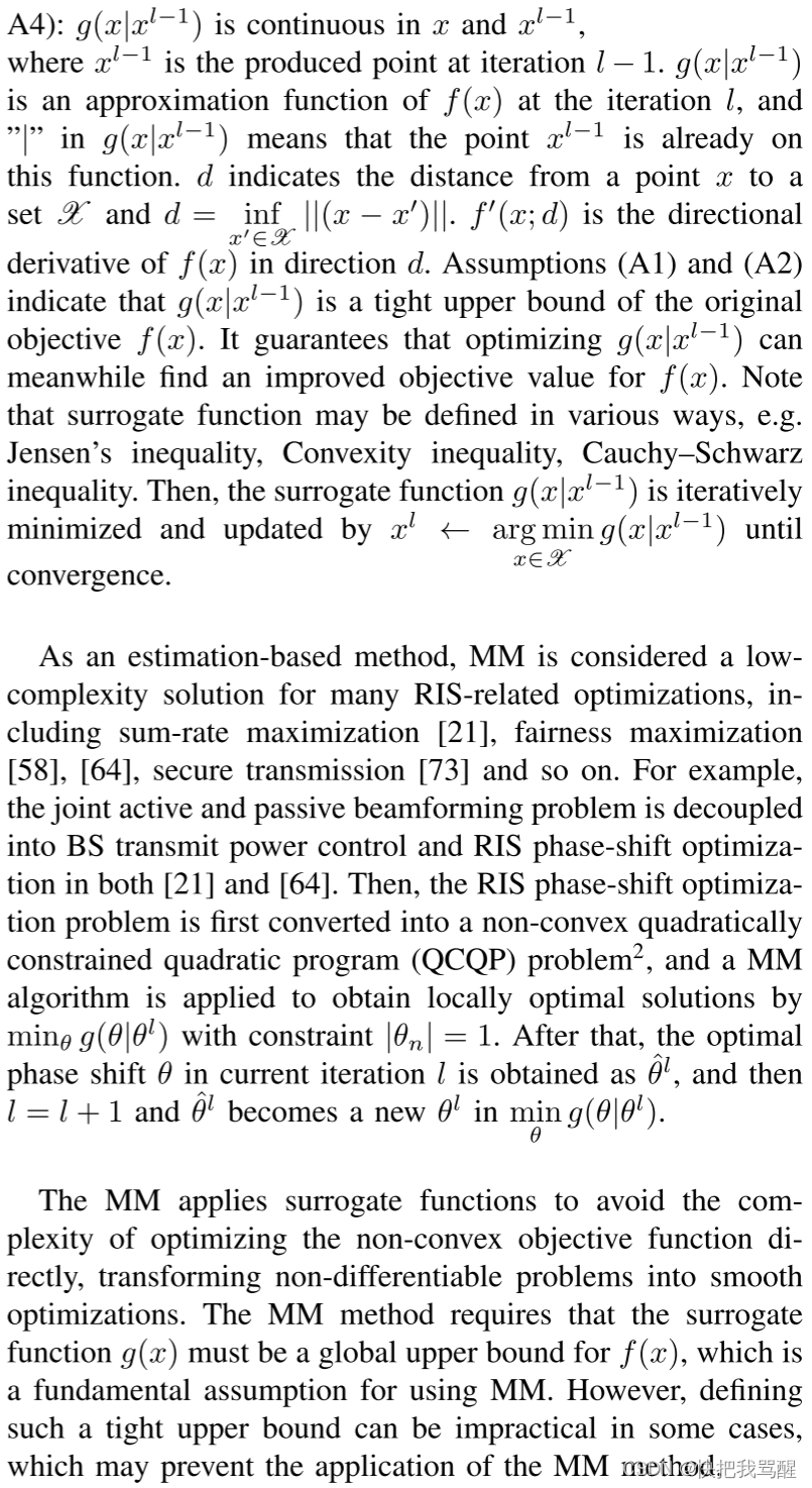
Majorization-Minimization Method(MM)

Successive Convex Approximation(SCA)

Similar to the MM algorithm, SCA applies a surrogate function $g(x)$ to approximate the original objective function $f(x)$ , which is shown in Fig. 6. However, the $g(x)$ in the SCA algorithm does not have to be a tight upper bound for $f(x)$ , reducing the complexity of the surrogate function design [93]. Therefore, SCA is more flexible and easier to be implemented for RIS-related optimization problems.
The SCA method first constructs a surrogate function $g(x)$ , and the assumptions are similar to the MM algorithm:
A1): $g\left(x\mid x^{l-1}\right)$ is continuous in $\mathcal{X}$ ;
A2): $g\left(x^{l-1}\mid x^{l-1}\right)=f(x)$ ;
A3): $g(x)$ is differentiable with ${{\nabla }_{x}g\left(x\mid x^{l-1}\right)|}_{x=x^{l-1}}={{\nabla }_{x}f(x)|}_{x=x^{l-1}}$ .
SCA relaxes the upper bound condition for the surrogate function, but $g\left(x\mid x^{l-1}\right)$ must be strongly convex in $\mathcal{X}$ . Then, solving the constructed surrogate problem $\underset{x\in \mathcal{X}}{\mathrm{argmin}}g\left(x\mid x^{l-1}\right)$ , and smoothing the next point by

$$x^l=x^{l-1}+{\beta }^{l-1}\left(\hat{\mathbf{x}}\left(x^l\right)-x^{l-1}\right)$$,

where ${\beta }^{l-1}$ is the step size for value updating. Finally, $g(x)$ construction and solving are repeated until meeting the convergence criteria. In SCA, the surrogate function $g(x)$ does not have to be a tight upper bound for $f(x)$ . Therefore, the step size in each iteration requires dedicated designs to guarantee an accurate approximation. The factor ${\beta }^{l-1}$ is used to control the $x^l$ updating step size. Meanwhile, the MM algorithm updates the whole control variable $x$ at each iteration, but SCA can be naturally implemented in a distributed manner when the constraints are separable.

Compared with MM, SCA is more frequently applied in RIS-related optimizations due to the relaxed upper bound, e.g., sum-rate maximization in [24], [29], [30] and power minimization in [41], [46]. Defining a surrogate function is the key to using the SCA method, which depends on specific objective functions and constraints in RIS-related applications. For instance, the non-convex BS transmit power constraint in [41] is replaced by a first-order Taylor approximation to apply the SCA algorithm. By contrast, Pan et al. in [11] claim that the unit modulus constraint of the RIS phase shift $\left|{\theta }_n\right|=1$ can be relaxed as a series of convex constraints, e.g., $1\le 2\mathrm{Re}\left\{{\theta }_n^{\ast }{\theta }_n^l\right\}-{\left|{\theta }_n^l\right|}^2$ , where Re ⁡ { ⋅ } \operatorname{Re}\{\cdot\} Re{⋅} denotes the real part of a complex argument and ${\theta }^{\ast }$ is the conjugate of \theta .

Semidefinite Relaxation(SR)

Many RIS-related signal processing problems can be described by QCQP formulations, and SDR is an efficient solution to solve QCQP problems [94]. The QCQP problem is defined by

$$\begin{array}{rl}\underset{x\in \mathcal{X}}{\min }& x^{T}Cx\\ \text{ s.t. }& x^T{D}_{i}x\ge b_i,i=1,2,3,,n,\end{array}\text{\hspace{1em}(12)}$$

where the " $\ge$ " in the constraint can also be replaced by " $\le$ " . Note that $x^{T}Cx$ produces an $1\times 1$ matrix, and therefore $x^{T}Cx=C{x}^{T}x=\mathrm{Tr}\left(C{x}^{T}x\right)$ . Similarly, $x^T{D}_{i}x=D_i{x}^{T}x=\mathrm{Tr}\left(D_i{x}^{T}x\right)$ is achieved. By introducing $X=x{x}^T$ , then

$$\begin{array}{rl}\underset{x\in \mathcal{X}}{\min }& \mathrm{Tr}(CX)\\ \text{ s.t. }& \mathrm{Tr}\left(D{X}_i\right)\ge b_i,i=1,2,3,,,I,\\ & X⪰0,\\ & \mathrm{rank}(X)=1,\end{array}\text{\hspace{1em}(13)}$$

where $Tr$ indicates the trace operation, and $X⪰0$ indicates that $X$ is positive semidefinite with $X=x{x}^T$ . Then, the nonconvex constraint $\mathrm{rank}(X)=1$ is relaxed and achieve

$$\begin{array}{rl}\underset{x\in \mathcal{X}}{\min }& \mathrm{Tr}(CX)\\ \text{ s.t. }& \mathrm{Tr}\left(D{X}_i\right)\ge b_i,i=1,2,3,,,I,\\ & X⪰0.\end{array}\text{\hspace{1em}(14)}$$

Equation (14) is an SDR of (13), which can be efficiently solved by semidefinite programming (SDP) [95]. SDR has been very generally applied to RIS-related optimization problems, since the $\mathrm{rank}(x)=1$ is frequently formulated for phase control. Specifically, the RIS phase shift constraint $\left|{\theta }_n\right|=1$ is non-convex with $\theta {\theta }^T=1$ . Then we can define $\mathcal{V}=\theta {\theta }^T$ with $\mathcal{V}⪰1$ and $\mathrm{rank}(\mathcal{V})=1$ , which can be then transformed and relaxed as shown by equations (13) and (14).

However, the main obstacle to applying SDR is to transform a globally optimal solution $\hat{\mathcal{V}}$ into a feasible solution $\hat{\theta }$ . An ideal solution is that $\hat{\mathcal{V}}$ is rank-one, and then $\hat{\theta }$ is easily obtained by solving $\hat{\mathcal{V}}=\hat{\theta }{\hat{\theta }}^T$ . Otherwise, if $\mathrm{rank}(\hat{\theta })>1$ , a rank-one approximation may be used to obtain a sub-optimal solution $\tilde{\theta }$ . There are multiple methods to find a feasible $\tilde{\theta }$ from $\hat{\mathcal{V}}$ , leading to various solution qualities. For instance, Mu et al. propose a penalty-based method to relax the rankone constraint, finding a sub-optimal solution by introducing penalties if $\mathrm{rank}(\hat{x})>1$ [4]. SDR has been used for sum-rate maximization [26], [34], [96], power minimization [40]-[42], [46], fairness maximization [37], [60], [63], [64], and secure transmission [67], [69], [70], [72], [74].

Second-order Cone Programming(SOCP)

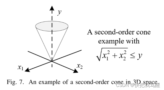
SOCP 是另一种用于有效解决无线网络优化问题的方法，尤其是 QCQP 和分数问题。图 7 展示了 3D 空间中的二阶锥体示例。 SOCP 是线性和二次规划的推广，允许将变量的仿射组合限制在二阶锥体内.

$$\begin{array}{l}{\min }_{x\in \mathcal{X}}{C}^{T}x\\ \text{ s.t. }\Vert A_{i}x+b_i\Vert \le c_i^{T}x+d_i,i=1,2,3,,,I\text{, }\end{array}$$

where $A\in {\mathbb{R}}^{n_i\times n}$, $b_i\in {\mathbb{R}}^{n_i}$, $c_i\in {\mathbb{R}}^n$, and $d_i\in \mathbb{R}$ . The $x$ in equation (15) may be RIS phase shifts, BS beamforming vectors, and so on, which depends on specific application scenarios. Consider the inverse image of the unit second-order cone with an affine mapping

$$\Vert A_{i}x+b_i\Vert \le c_i^{T}x+d_i\leftrightarrow \left[\begin{array}{c}{A}_i\\ c_i^T\end{array}\right]x+\left[\begin{array}{c}{b}_i\\ d_i\end{array}\right]\in {\mathcal{C}}_{n_i+1}$$

Therefore, SOCP is a convex optimization problem with a convex objective function and convex constraints. Equation (16) indicates the core properties of SOCP problems, and hence many problems are converted into SOCPs and solved efficiently [97].

For instance, sum and fractional problems are frequently defined in RIS-related problems to maximize the sum-rate or total throughput regarding the SINR

$$\begin{array}{cl}{\min }_{x\in \mathcal{X}}& {\sum }_{i=1}^I\frac{{\Vert C_i^T+D_i\Vert }^2}{A_i^{T}x+B_i}\\ \text{ s.t. }& A_i^{T}x+B_i\ge 0,i=1,2,3,,,I,\end{array}$$

which is converted into a SOCP by

$$\begin{array}{cl}{\min }_{x\in \mathcal{X}}& {\sum }_{i=1}^I{t}_i\\ \text{ s.t. }& {\left(C_i^T+D_i\right)}^T\left(C_i^T+D_i\right)\le t_i\left(A_i^{T}x+B_i\right),\\ & A_i^{T}x+B_i>0,i=1,2,3,,,I.\end{array}$$

SOCP can be efficiently solved by the interior point method. Meanwhile, SOCP is less general than SDP since equation (15) may be transformed into an SDP problem. However, the complexity of solving SOCP is $O\left(n^2{\sum }_i{n}_i\right)$ , while the complexity for SDP is $O\left(n^2{\sum }_i{n}_i^2\right)$ [98]. Such complexity difference is crucial for large-dimension problems.

Finally, to apply SOCP for RIS-aided optimizations, the first step is to utilize AO or BCD scheme to decouple the control variables into multiple sub-problems, e.g., BS precoding matrix and RIS passive beamforming [44], [58], [64], coordinated transmit beamforming and RIS passive beamforming [60]. For example, the max-min data rate problem in [64] is decoupled into SOCP-based BS beamforming and SDR-based RIS phaseshift control, and the data rate maximization problem in [25] is converted into a SOCP-based BS active beamforming and SDR-based RIS passive beamforming.

Fractional Programming(FP)

Branch-and-Bound(BnB) 分支界定

HEURISTIC ALGORITHMS FOR RIS-AIDED WIRELESS NETWORKS

A Convex-concave Procedure

B Meta-heuristic Algorithms

C Greedy Algorithms

D Matching Theory-based Methods

E Discussions and Numerical Results

ML-ENABLED OPTIMIZATION FOR RIS-AIDED WIRELESS NETWORKS

A Supervised Learning-enabled Optimization

1 Dataset Acquisition in RIS-aided Environments:

2 Loss Functions and Algorithm Training

3 Neural Network Architecture and Overfitting

B Unsupervised Learning-based Optimization

这篇关于RIS 辅助无线网络：基于模型、启发式和机器学习の优化方法的文章就介绍到这儿，希望我们推荐的文章对编程师们有所帮助！

---