本文主要是介绍企业级实战项目:基于 pycaret 自动化预测公司是否破产,希望对大家解决编程问题提供一定的参考价值,需要的开发者们随着小编来一起学习吧!
本文系数据挖掘实战系列文章,我跟大家分享一个数据挖掘实战,与以往的数据实战不同的是,用自动机器学习方法完成模型构建与调优部分工作,深入理解由此带来的便利与效果。
1. Introduction
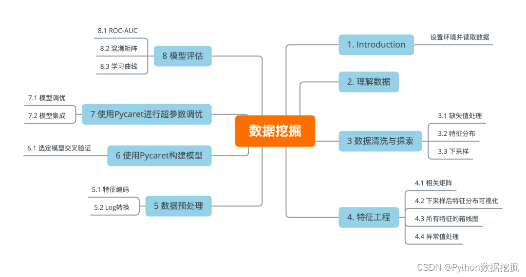
本文是一篇数据挖掘实战案例,详细探索了从台湾经济杂志收集的1999年到2009年的数据,看看在数据探索过程中,可以洞察出哪些有用的信息,判断哪一个模型能够最准确地预测公司是否破产。
公司破产的定义是根据台湾证券交易所的商业规则而定的。
该建模将尝试使用自动机器学习库pycaret来构建机器学习模型,pycaret是一个用python编写的开源低代码机器学习库,它将机器学习工作流程自动化。如果你想探索这个库并更好地理解它的功能。推荐查看
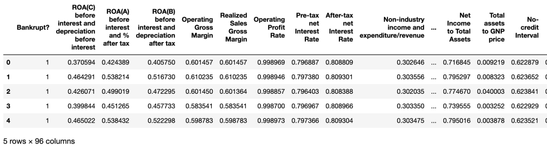
设置环境并读取数据
import pandas as pd
import numpy as np
import math
import matplotlib.pyplot as plt
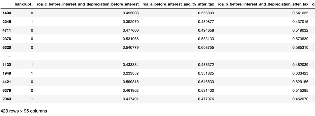
import seaborn as sns bankruptcy_df = pd.read_csv("Bankruptcy.csv") bankruptcy_df.head()
技术交流&源码获取
技术要学会交流、分享,不建议闭门造车。一个人可以走的很快、一堆人可以走的更远。
好的文章离不开粉丝的分享、推荐,资料干货、资料分享、数据、技术交流提升,均可加交流群获取,群友已超过2000人,添加时最好的备注方式为:来源+兴趣方向,方便找到志同道合的朋友。
本文数据&源码,技术交流、按照如下方式获取:
方式①、添加微信号:dkl88194,备注:资料
方式②、微信搜索公众号:Python学习与数据挖掘,后台回复:资料
资料1

资料2
我们打造了《100个超强算法模型》,特点:从0到1轻松学习,原理、代码、案例应有尽有,所有的算法模型都是按照这样的节奏进行表述,所以是一套完完整整的案例库。
很多初学者是有这么一个痛点,就是案例,案例的完整性直接影响同学的兴致。因此,我整理了 100个最常见的算法模型,在你的学习路上助推一把!

2. 理解数据
bankruptcy_df.info()
<class 'pandas.core.frame.DataFrame'>
RangeIndex: 6819 entries, 0 to 6818
Data columns (total 96 columns):  #   Column                                                    Non-Null Count  Dtype    ---  ------                                                    --------------  -----  0   Bankrupt?                                                 6819 non-null   int64    1    ROA(C) before interest and depreciation before interest  6819 non-null   float64  2    ROA(A) before interest and % after tax                   6819 non-null   float64  3    ROA(B) before interest and depreciation after tax        6819 non-null   float64  4    Operating Gross Margin                                   6819 non-null   float64  5    Realized Sales Gross Margin                              6819 non-null   float64  6    Operating Profit Rate                                    6819 non-null   float64  7    Pre-tax net Interest Rate                                6819 non-null   float64  8    After-tax net Interest Rate                              6819 non-null   float64  9    Non-industry income and expenditure/revenue              6819 non-null   float64  10   Continuous interest rate (after tax)                     6819 non-null   float64  11   Operating Expense Rate                                   6819 non-null   float64  12   Research and development expense rate                    6819 non-null   float64  13   Cash flow rate                                           6819 non-null   float64  14   Interest-bearing debt interest rate                      6819 non-null   float64  15   Tax rate (A)                                             6819 non-null   float64  16   Net Value Per Share (B)                                  6819 non-null   float64  17   Net Value Per Share (A)                                  6819 non-null   float64  18   Net Value Per Share (C)                                  6819 non-null   float64  19   Persistent EPS in the Last Four Seasons                  6819 non-null   float64  20   Cash Flow Per Share                                      6819 non-null   float64  21   Revenue Per Share (Yuan ¥)                               6819 non-null   float64  22   Operating Profit Per Share (Yuan ¥)                      6819 non-null   float64  23   Per Share Net profit before tax (Yuan ¥)                 6819 non-null   float64  24   Realized Sales Gross Profit Growth Rate                  6819 non-null   float64  25   Operating Profit Growth Rate                             6819 non-null   float64  26   After-tax Net Profit Growth Rate                         6819 non-null   float64  27   Regular Net Profit Growth Rate                           6819 non-null   float64  28   Continuous Net Profit Growth Rate                        6819 non-null   float64  29   Total Asset Growth Rate                                  6819 non-null   float64  30   Net Value Growth Rate                                    6819 non-null   float64  31   Total Asset Return Growth Rate Ratio                     6819 non-null   float64  32   Cash Reinvestment %                                      6819 non-null   float64  33   Current Ratio                                            6819 non-null   float64  34   Quick Ratio                                              6819 non-null   float64  35   Interest Expense Ratio                                   6819 non-null   float64  36   Total debt/Total net worth                               6819 non-null   float64  37   Debt ratio %                                             6819 non-null   float64  38   Net worth/Assets                                         6819 non-null   float64  39   Long-term fund suitability ratio (A)                     6819 non-null   float64  40   Borrowing dependency                                     6819 non-null   float64  41   Contingent liabilities/Net worth                         6819 non-null   float64  42   Operating profit/Paid-in capital                         6819 non-null   float64  43   Net profit before tax/Paid-in capital                    6819 non-null   float64  44   Inventory and accounts receivable/Net value              6819 non-null   float64  45   Total Asset Turnover                                     6819 non-null   float64  46   Accounts Receivable Turnover                             6819 non-null   float64  47   Average Collection Days                                  6819 non-null   float64  48   Inventory Turnover Rate (times)                          6819 non-null   float64  49   Fixed Assets Turnover Frequency                          6819 non-null   float64  50   Net Worth Turnover Rate (times)                          6819 non-null   float64  51   Revenue per person                                       6819 non-null   float64  52   Operating profit per person                              6819 non-null   float64  53   Allocation rate per person                               6819 non-null   float64  54   Working Capital to Total Assets                          6819 non-null   float64  55   Quick Assets/Total Assets                                6819 non-null   float64  56   Current Assets/Total Assets                              6819 non-null   float64  57   Cash/Total Assets                                        6819 non-null   float64  58   Quick Assets/Current Liability                           6819 non-null   float64  59   Cash/Current Liability                                   6819 non-null   float64  60   Current Liability to Assets                              6819 non-null   float64  61   Operating Funds to Liability                             6819 non-null   float64  62   Inventory/Working Capital                                6819 non-null   float64  63   Inventory/Current Liability                              6819 non-null   float64  64   Current Liabilities/Liability                            6819 non-null   float64  65   Working Capital/Equity                                   6819 non-null   float64  66   Current Liabilities/Equity                               6819 non-null   float64  67   Long-term Liability to Current Assets                    6819 non-null   float64  68   Retained Earnings to Total Assets                        6819 non-null   float64  69   Total income/Total expense                               6819 non-null   float64  70   Total expense/Assets                                     6819 non-null   float64  71   Current Asset Turnover Rate                              6819 non-null   float64  72   Quick Asset Turnover Rate                                6819 non-null   float64  73   Working capitcal Turnover Rate                           6819 non-null   float64  74   Cash Turnover Rate                                       6819 non-null   float64  75   Cash Flow to Sales                                       6819 non-null   float64  76   Fixed Assets to Assets                                   6819 non-null   float64  77   Current Liability to Liability                           6819 non-null   float64  78   Current Liability to Equity                              6819 non-null   float64  79   Equity to Long-term Liability                            6819 non-null   float64  80   Cash Flow to Total Assets                                6819 non-null   float64  81   Cash Flow to Liability                                   6819 non-null   float64  82   CFO to Assets                                            6819 non-null   float64  83   Cash Flow to Equity                                      6819 non-null   float64  84   Current Liability to Current Assets                      6819 non-null   float64  85   Liability-Assets Flag                                    6819 non-null   int64    86   Net Income to Total Assets                               6819 non-null   float64  87   Total assets to GNP price                                6819 non-null   float64  88   No-credit Interval                                       6819 non-null   float64  89   Gross Profit to Sales                                    6819 non-null   float64  90   Net Income to Stockholder's Equity                       6819 non-null   float64  91   Liability to Equity                                      6819 non-null   float64  92   Degree of Financial Leverage (DFL)                       6819 non-null   float64  93   Interest Coverage Ratio (Interest expense to EBIT)       6819 non-null   float64  94   Net Income Flag                                          6819 non-null   int64    95   Equity to Liability                                      6819 non-null   float64
dtypes: float64(93), int64(3)
memory usage: 5.0 MB
bankruptcy_df.shape
(6819, 96)
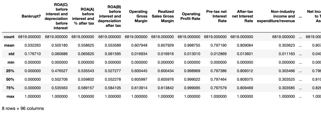
bankruptcy_df.describe()
3. 数据探索与清洗
3.1 缺失值处理
bankruptcy_df.columns[bankruptcy_df.isna().any()]
Index([], dtype='object')
从结果看,改数据集非常完整,没有缺失值!
.any()指的是有没有(缺失值),而与之对应的.all()指的是是否都是(缺失值)
调整数据列名
def clean_col_names(col_name):  col_name = (  col_name.strip()  .replace("?", "_")  .replace("(", "_")  .replace(")", "_")  .replace(" ", "_")  .replace("/", "_")  .replace("-", "_")  .replace("__", "_")  .replace("'", "")  .lower()  )  return col_name  bank_columns = list(bankruptcy_df.columns)
bank_columns = [clean_col_names(col_name) for col_name in bank_columns]
bankruptcy_df.columns = bank_columns
display(bankruptcy_df.columns)
Index(['bankrupt_', 'roa_c_before_interest_and_depreciation_before_interest', 'roa_a_before_interest_and_%_after_tax', 'roa_b_before_interest_and_depreciation_after_tax', 'operating_gross_margin', 'realized_sales_gross_margin', 'operating_profit_rate', 'pre_tax_net_interest_rate', 'after_tax_net_interest_rate', 'non_industry_income_and_expenditure_revenue', 'continuous_interest_rate_after_tax_', 'operating_expense_rate', 'research_and_development_expense_rate', 'cash_flow_rate', 'interest_bearing_debt_interest_rate', 'tax_rate_a_', 'net_value_per_share_b_', 'net_value_per_share_a_', 'net_value_per_share_c_', 'persistent_eps_in_the_last_four_seasons', 'cash_flow_per_share', 'revenue_per_share_yuan_¥_', 'operating_profit_per_share_yuan_¥_', 'per_share_net_profit_before_tax_yuan_¥_', 'realized_sales_gross_profit_growth_rate', 'operating_profit_growth_rate', 'after_tax_net_profit_growth_rate', 'regular_net_profit_growth_rate', 'continuous_net_profit_growth_rate', 'total_asset_growth_rate', 'net_value_growth_rate', 'total_asset_return_growth_rate_ratio', 'cash_reinvestment_%', 'current_ratio', 'quick_ratio', 'interest_expense_ratio', 'total_debt_total_net_worth', 'debt_ratio_%', 'net_worth_assets', 'long_term_fund_suitability_ratio_a_', 'borrowing_dependency', 'contingent_liabilities_net_worth', 'operating_profit_paid_in_capital', 'net_profit_before_tax_paid_in_capital', 'inventory_and_accounts_receivable_net_value', 'total_asset_turnover', 'accounts_receivable_turnover', 'average_collection_days', 'inventory_turnover_rate_times_', 'fixed_assets_turnover_frequency', 'net_worth_turnover_rate_times_', 'revenue_per_person', 'operating_profit_per_person', 'allocation_rate_per_person', 'working_capital_to_total_assets', 'quick_assets_total_assets', 'current_assets_total_assets', 'cash_total_assets', 'quick_assets_current_liability', 'cash_current_liability', 'current_liability_to_assets', 'operating_funds_to_liability', 'inventory_working_capital', 'inventory_current_liability', 'current_liabilities_liability', 'working_capital_equity', 'current_liabilities_equity', 'long_term_liability_to_current_assets', 'retained_earnings_to_total_assets', 'total_income_total_expense', 'total_expense_assets', 'current_asset_turnover_rate', 'quick_asset_turnover_rate', 'working_capitcal_turnover_rate', 'cash_turnover_rate', 'cash_flow_to_sales', 'fixed_assets_to_assets', 'current_liability_to_liability', 'current_liability_to_equity', 'equity_to_long_term_liability', 'cash_flow_to_total_assets', 'cash_flow_to_liability', 'cfo_to_assets', 'cash_flow_to_equity', 'current_liability_to_current_assets', 'liability_assets_flag', 'net_income_to_total_assets', 'total_assets_to_gnp_price', 'no_credit_interval', 'gross_profit_to_sales', 'net_income_to_stockholders_equity', 'liability_to_equity', 'degree_of_financial_leverage_dfl_', 'interest_coverage_ratio_interest_expense_to_ebit_', 'net_income_flag', 'equity_to_liability'], dtype='object')
统计并绘制目标变量
该步骤的目的是查看目标变量是否平衡,如果不平衡,则需要针对性处理。
class_bar=sns.countplot(data=bankruptcy_df,x="bankrupt_")
ax = plt.gca()
for p in ax.patches:  ax.annotate('{:.1f}'.format(p.get_height()), (p.get_x()+0.3, p.get_height()+500))
class_bar
3.2 特征分布
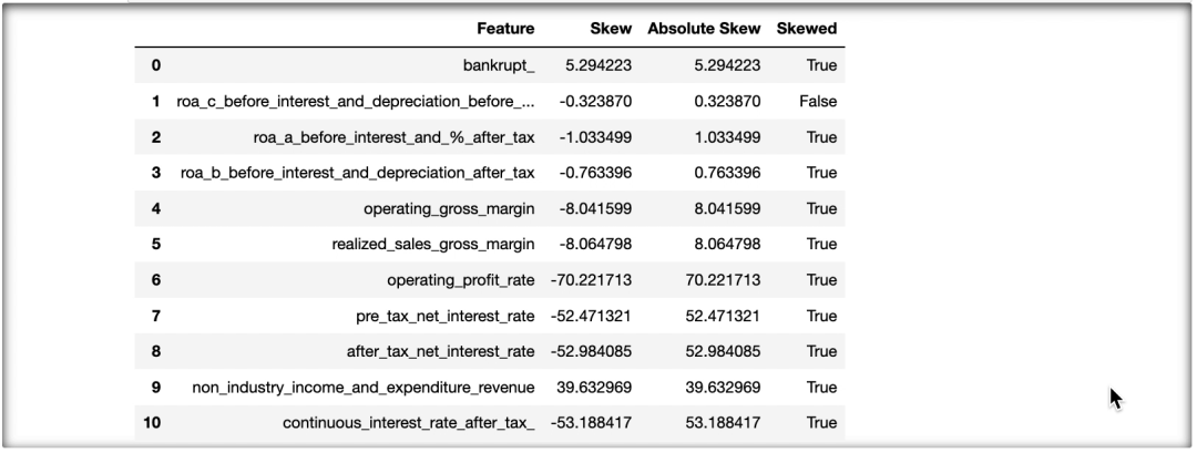
检查偏态
# Return true/false if skewed
import scipy.stats
skew_df = pd.DataFrame(bankruptcy_df.select_dtypes(np.number).columns, columns = ['Feature'])  skew_df['Skew'] = skew_df['Feature'].apply(lambda feature: scipy.stats.skew(bankruptcy_df[feature]))   skew_df['Absolute Skew'] = skew_df['Skew'].apply(abs)
# 得到与方向无关的倾斜幅度
skew_df['Skewed']= skew_df['Absolute Skew'].apply(lambda x: True if x>= 0.5 else False)
with pd.option_context("display.max_rows", 1000):  display(skew_df)
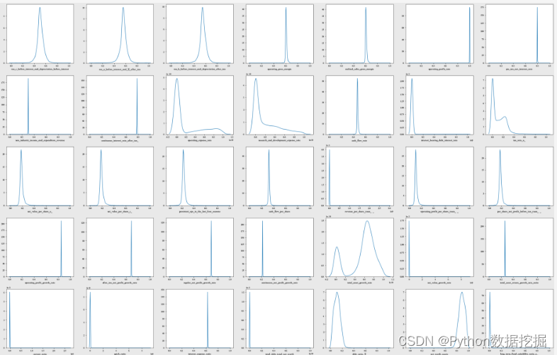
可视化分布
cols = list(bankruptcy_df.columns)
ncols = 8
nrows = math.ceil(len(cols) / ncols)  fig, ax = plt.subplots(nrows, ncols, figsize = (4.5 * ncols, 4 * nrows))
for i in range(len(cols)):  sns.kdeplot(bankruptcy_df[cols[i]], ax = ax[i // ncols, i % ncols])  if i % ncols != 0:  ax[i // ncols, i % ncols].set_ylabel(" ")
plt.tight_layout()
plt.show()
查看有偏态的特征
query_skew=skew_df.query("Skewed == True")["Feature"]
with pd.option_context("display.max_rows", 1000):  display(query_skew)
0                                             bankrupt_
2                 roa_a_before_interest_and_%_after_tax
3      roa_b_before_interest_and_depreciation_after_tax
4                                operating_gross_margin
5                           realized_sales_gross_margin
6                                 operating_profit_rate
7                             pre_tax_net_interest_rate
8                           after_tax_net_interest_rate
9           non_industry_income_and_expenditure_revenue
10                  continuous_interest_rate_after_tax_
11                               operating_expense_rate
12                research_and_development_expense_rate
13                                       cash_flow_rate
14                  interest_bearing_debt_interest_rate
15                                          tax_rate_a_
16                               net_value_per_share_b_
17                               net_value_per_share_a_
18                               net_value_per_share_c_
19              persistent_eps_in_the_last_four_seasons
20                                  cash_flow_per_share
21                            revenue_per_share_yuan_¥_
22                   operating_profit_per_share_yuan_¥_
23              per_share_net_profit_before_tax_yuan_¥_
24              realized_sales_gross_profit_growth_rate
25                         operating_profit_growth_rate
26                     after_tax_net_profit_growth_rate
27                       regular_net_profit_growth_rate
28                    continuous_net_profit_growth_rate
29                              total_asset_growth_rate
30                                net_value_growth_rate
31                 total_asset_return_growth_rate_ratio
32                                  cash_reinvestment_%
33                                        current_ratio
34                                          quick_ratio
35                               interest_expense_ratio
36                           total_debt_total_net_worth
37                                         debt_ratio_%
38                                     net_worth_assets
39                  long_term_fund_suitability_ratio_a_
40                                 borrowing_dependency
41                     contingent_liabilities_net_worth
42                     operating_profit_paid_in_capital
43                net_profit_before_tax_paid_in_capital
44          inventory_and_accounts_receivable_net_value
45                                 total_asset_turnover
46                         accounts_receivable_turnover
47                              average_collection_days
48                       inventory_turnover_rate_times_
49                      fixed_assets_turnover_frequency
50                       net_worth_turnover_rate_times_
51                                   revenue_per_person
52                          operating_profit_per_person
53                           allocation_rate_per_person
57                                    cash_total_assets
58                       quick_assets_current_liability
59                               cash_current_liability
60                          current_liability_to_assets
61                         operating_funds_to_liability
62                            inventory_working_capital
63                          inventory_current_liability
64                        current_liabilities_liability
65                               working_capital_equity
66                           current_liabilities_equity
67                long_term_liability_to_current_assets
68                    retained_earnings_to_total_assets
69                           total_income_total_expense
70                                 total_expense_assets
71                          current_asset_turnover_rate
72                            quick_asset_turnover_rate
73                       working_capitcal_turnover_rate
74                                   cash_turnover_rate
75                                   cash_flow_to_sales
76                               fixed_assets_to_assets
77                       current_liability_to_liability
78                          current_liability_to_equity
79                        equity_to_long_term_liability
81                               cash_flow_to_liability
83                                  cash_flow_to_equity
84                  current_liability_to_current_assets
85                                liability_assets_flag
86                           net_income_to_total_assets
87                            total_assets_to_gnp_price
88                                   no_credit_interval
89                                gross_profit_to_sales
90                    net_income_to_stockholders_equity
91                                  liability_to_equity
92                    degree_of_financial_leverage_dfl_
93    interest_coverage_ratio_interest_expense_to_ebit_
95                                  equity_to_liability
Name: Feature, dtype: object
进行下采样,直至样本集中的破产与非破产比例为50/50。完成之后再次对数据进行偏态检查,决定是否需要做log转换,另外进行相关矩阵分析。
3.3 下采样
首先对数据集进行下采样,目标比例为bankrupt vs non bankrupt = 50 vs 50。
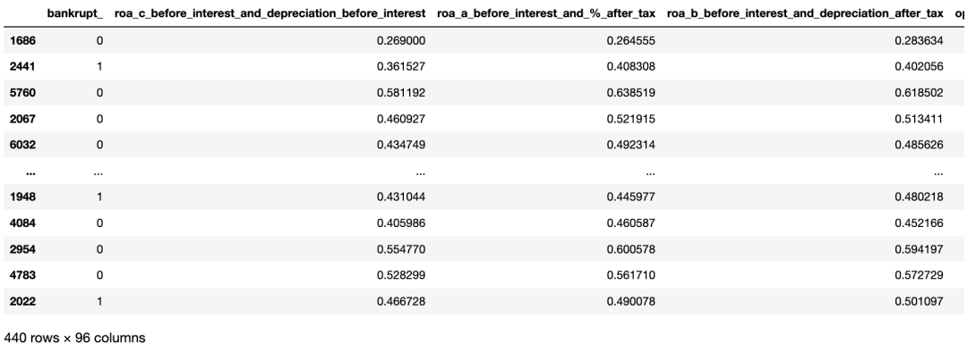
bankruptcy_df2 = bankruptcy_df.sample(frac=1) #Shuffle Bankruptcy df  bankruptcy_df_b = bankruptcy_df2.loc[bankruptcy_df2["bankrupt_"] == 1]
bankruptcy_df_nb = bankruptcy_df2.loc[bankruptcy_df2["bankrupt_"] == 0][:220]  bankruptcy_subdf_comb = pd.concat([bankruptcy_df_b,bankruptcy_df_nb])
bankruptcy_subdf = bankruptcy_subdf_comb.sample(frac=1,random_state=42)  bankruptcy_subdf
再次绘图查看正负样本数。
sns.countplot(bankruptcy_subdf["bankrupt_"])
随机选择220家非破产公司和220家破产公司。
4. 特征工程
bankruptcy_subdf2 = bankruptcy_subdf.drop(["net_income_flag"],axis=1)
bankruptcy_subdf2.shape
(440, 95)
4.1 相关矩阵
fig = plt.figure(figsize=(30,20))
ax1 = fig.add_subplot(1,1,1)
sns.heatmap(bankruptcy_subdf2.corr(),ax=ax1,cmap="coolwarm")
4.1.1 找出与破产相关的最高特征
根据对破产企业的基本认识,破产企业资产少、负债高、盈利能力低、现金流少。可以朝这个方向分析我们的数据集。
corr=bankruptcy_subdf2[bankruptcy_subdf2.columns[:-1]].corr()['bankrupt_'][:]  corr_df = pd.DataFrame(corr)  print("Correlations to Bankruptcy:")
for index, row in corr_df["bankrupt_"].iteritems():  if row!=1.0 and row>=0.5:  print(f'Positive Correlation: {index}')  elif row!=1.0 and row<=-0.5:  print(f'Negative Correlation: {index}')
Correlations to Bankruptcy:
Negative Correlation: roa_c_before_interest_and_depreciation_before_interest
Negative Correlation: roa_b_before_interest_and_depreciation_after_tax
Negative Correlation: net_value_per_share_b_
Negative Correlation: net_value_per_share_a_
Negative Correlation: net_value_per_share_c_
Negative Correlation: persistent_eps_in_the_last_four_seasons
Negative Correlation: per_share_net_profit_before_tax_yuan_¥_
Positive Correlation: debt_ratio_%
Negative Correlation: net_worth_assets
Negative Correlation: net_profit_before_tax_paid_in_capital
Negative Correlation: total_income_total_expense
这些特征代表什么
-
roa_c_before_interest_and_depreciation_before_interest息前资产收益率和息前折旧:总资产收益率–如果总资产收益率低,破产风险高
-
roa_a_before_interest_and_after_tax息前和税后利润:总资产回报率–如果总资产回报率较低,破产风险较高
-
roa_b_before_interest_and_depreciation_after_tax利润不计利息及税后折旧:总资产回报率–如果总资产回报率较低,破产风险较高
-
debt_ratio负债率:负债占总资产的比例–价值越高,负债占资产的比例越高,导致破产风险越高
-
net_worth_assets净资产:净资产越少,破产风险越高
-
retained_earnings_to_total_assets留存收益与总资产之比:留存收益越少,破产风险越高
-
total_income_total_expense总费用:收入与费用之比较低,破产风险较高
-
net_income_to_total_assets净收入与总资产之比:净收入越低,破产风险越高
从结果看,导致公司违约风险越高的特征,似乎与背景知识一致。
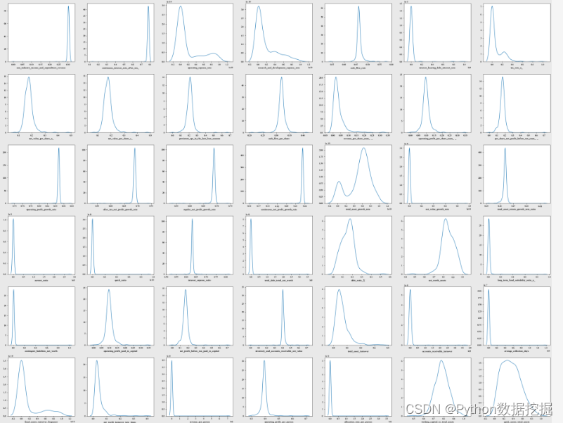
4.2 下采样后特征分布可视化
# Visualisation of distributions after sub-sampling
cols = list(bankruptcy_subdf2.columns)
ncols = 8
nrows = math.ceil(len(cols) / ncols)  fig, ax = plt.subplots(nrows, ncols, figsize = (4.5 * ncols, 4 * nrows))
for i in range(len(cols)):  sns.kdeplot(bankruptcy_subdf2[cols[i]], ax = ax[i // ncols, i % ncols])  if i % ncols != 0:  ax[i // ncols, i % ncols].set_ylabel(" ")
plt.tight_layout()
plt.show()
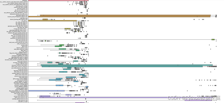
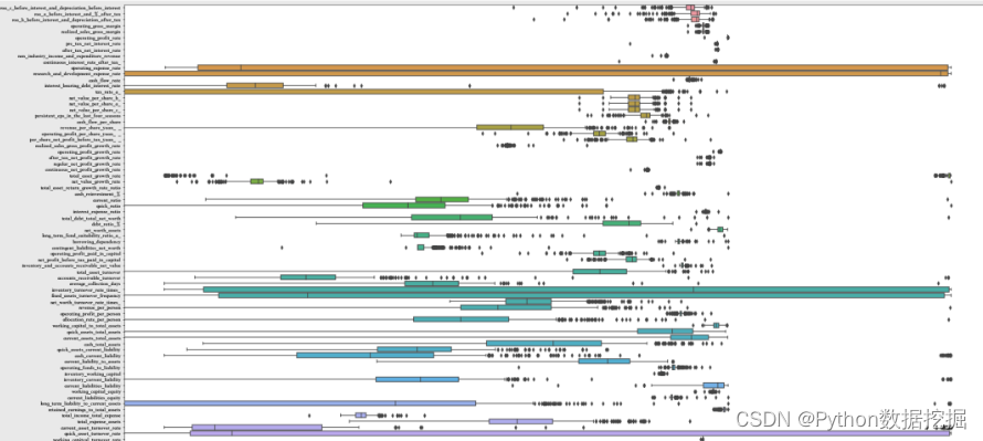
4.3 所有特征的箱线图
plt.figure(figsize=(30,20))
boxplot=sns.boxplot(data=bankruptcy_subdf2,orient="h")
boxplot.set(xscale="log")
plt.show()
4.4 异常值处理
quartile1 = bankruptcy_subdf2.quantile(q=0.25,axis=0)
# display(quartile1)
quartile3 = bankruptcy_subdf2.quantile(q=0.75,axis=0)
# display(quartile3)
IQR = quartile3 -quartile1
lower_limit = quartile1-1.5*IQR
upper_limit = quartile3+1.5*IQR  lower_limit = lower_limit.drop(["bankrupt_"])
upper_limit = upper_limit.drop(["bankrupt_"])
# print(lower_limit)
# print(" ")
# print(upper_limit)  bankruptcy_subdf2_out = bankruptcy_subdf2[((bankruptcy_subdf2<lower_limit) | (bankruptcy_subdf2>upper_limit)).any(axis=1)]
display(bankruptcy_subdf2_out.shape)
display(bankruptcy_subdf2.shape)
(423, 95) (440, 95)
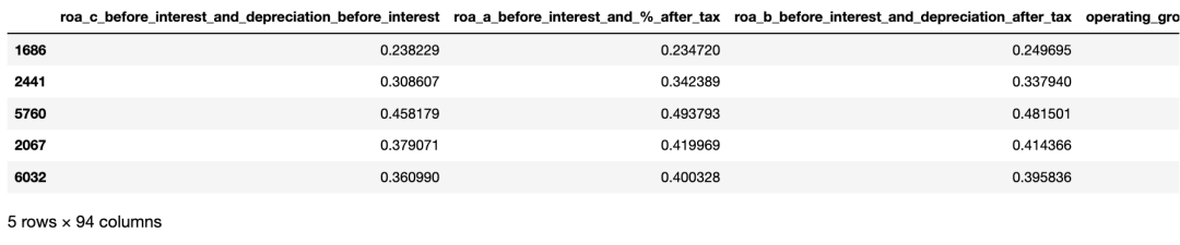
额外复制一份表,供后续分析处理。
bankruptcy_subdf3 = bankruptcy_subdf2_out.copy()
bankruptcy_subdf3
下采样后且去除离群值后的分布可视化。
# Visualisation of distributions after sub-sampling after outlier removal
cols = list(bankruptcy_subdf3.columns)
ncols = 8
nrows = math.ceil(len(cols) / ncols)  fig, ax = plt.subplots(nrows, ncols, figsize = (4.5 * ncols, 4 * nrows))
for i in range(len(cols)):  sns.kdeplot(bankruptcy_subdf3[cols[i]], ax = ax[i // ncols, i % ncols],fill=True,color="red")  sns.kdeplot(bankruptcy_subdf2[cols[i]], ax = ax[i // ncols, i % ncols],color="green")  if i % ncols != 0:  ax[i // ncols, i % ncols].set_ylabel(" ")
plt.tight_layout()
plt.show() 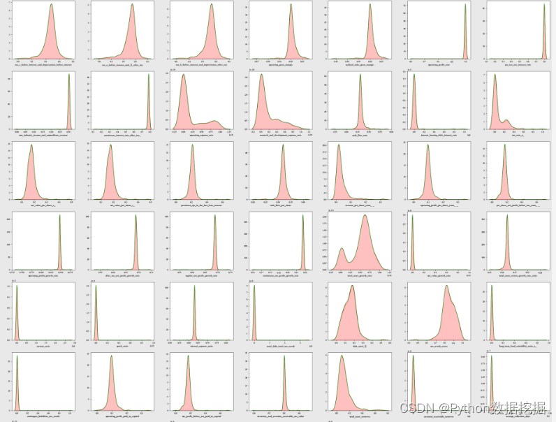
5 数据预处理
5.1 特征编码
所有类别在基础数据中都已编码完成,因此这里不需要再次编码列。在实际工作中,这一步大概率是必不可少的,编码技术也是尤其重要,需要好好掌握。如果你还不了解或不是很了解,推荐查看:
5.2 Log转换
这一步是为了去除数据中的偏态分布。
# Log transform to remove skews
target = bankruptcy_subdf3['bankrupt_']
bankruptcy_subdf4 = bankruptcy_subdf3.drop(["bankrupt_"],axis=1)  def log_trans(data):  for col in data:  skew = data[col].skew()  if skew>=0.5 or skew<=0.5:  data[col] = np.log1p(data[col])  else:  continue  return data  bankruptcy_subdf4_log = log_trans(bankruptcy_subdf4)
bankruptcy_subdf4_log.head()
5.2.1 Log转换数据的箱线图
plt.figure(figsize=(30,20))
boxplot=sns.boxplot(data=bankruptcy_subdf4_log,orient="h")
boxplot.set(xscale="log")
plt.show()
5.2.2 Log转换后的数据分布可视化
# 在下采样后、去除离群值及log变换后的数据分布的可视化
compare_subdf2 = bankruptcy_subdf2.drop(["bankrupt_"],axis=1)  cols = list(bankruptcy_subdf4.columns)
ncols = 8
nrows = math.ceil(len(cols) / ncols)  fig, ax = plt.subplots(nrows, ncols, figsize = (4.5 * ncols, 4 * nrows))
for i in range(len(cols)):  sns.kdeplot(bankruptcy_subdf4_log[cols[i]], ax = ax[i // ncols, i % ncols],fill=True,color="red")  sns.kdeplot(bankruptcy_subdf2[cols[i]], ax = ax[i // ncols, i % ncols],color="green")  if i % ncols != 0:  ax[i // ncols, i % ncols].set_ylabel(" ")
plt.tight_layout()
plt.show()
print("Red represents distributions after log transforms, green represents before log transform")
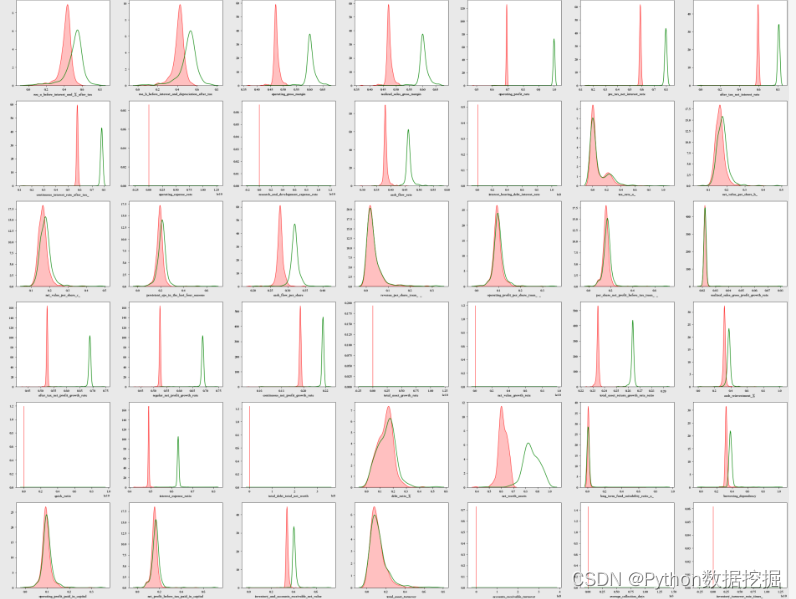
红色表示Log变换后的分布,绿色表示Log变换前的分布。(完整数据集:关注@公众号:数据STUDIO,联系云朵君获取)
6 使用Pycaret构建模型
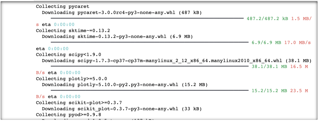
本次模型构建使用的是自动机器学习框架pycaret,如果你还没有安装,可使用下述命令安装即可。
pip install -U --ignore-installed --pre pycaret
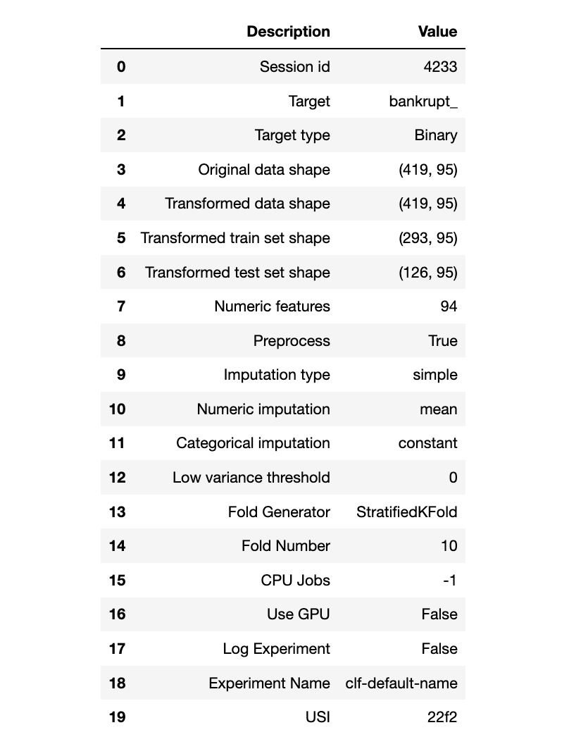
在pycaret中自动完成训练及测试数据的切分工作。
from pycaret.classification import *
exp_name = setup(data = bankruptcy_subdf4,  target = bankruptcy_subdf3["bankrupt_"])
compare_models()
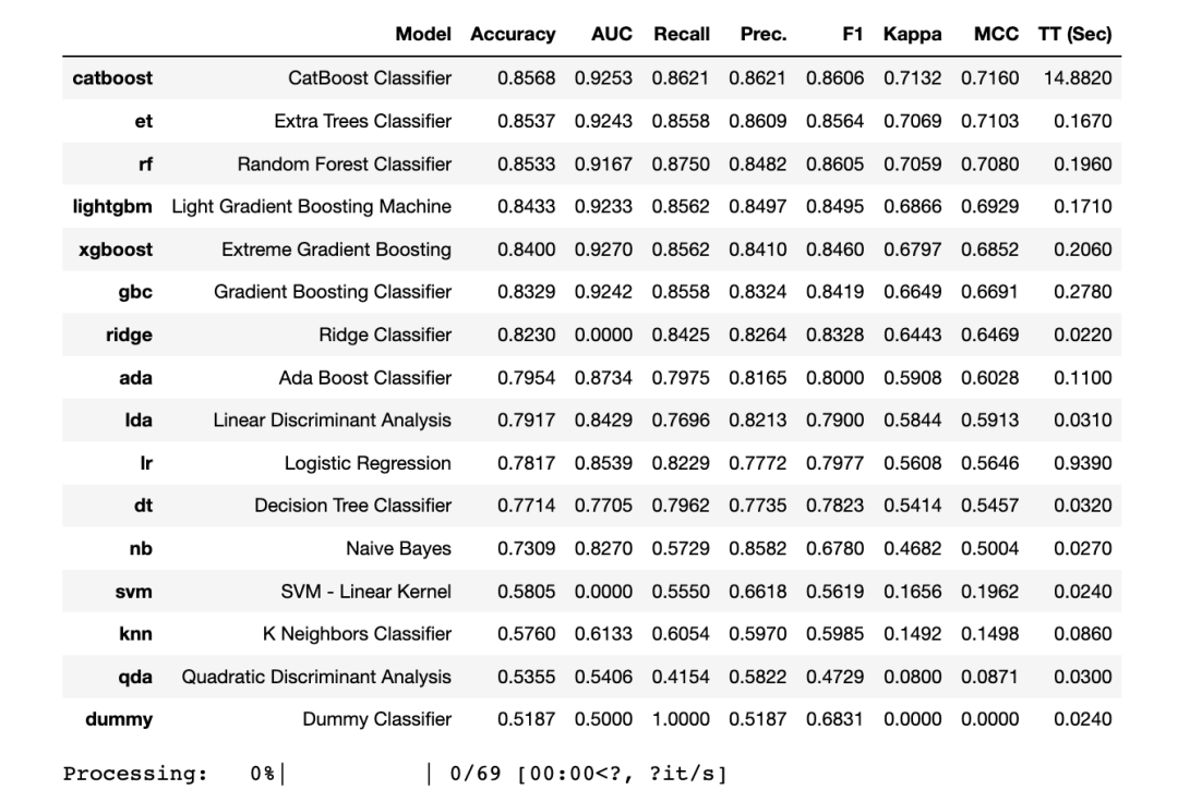
Pycaret显示,3种模型的准确性最高的是
-
LightGBM分类器
-
梯度提升GBC分类器
-
XGBoost分类器
接下来将使用这5个模型进行超参数调优。
6.1 选定模型交叉验证
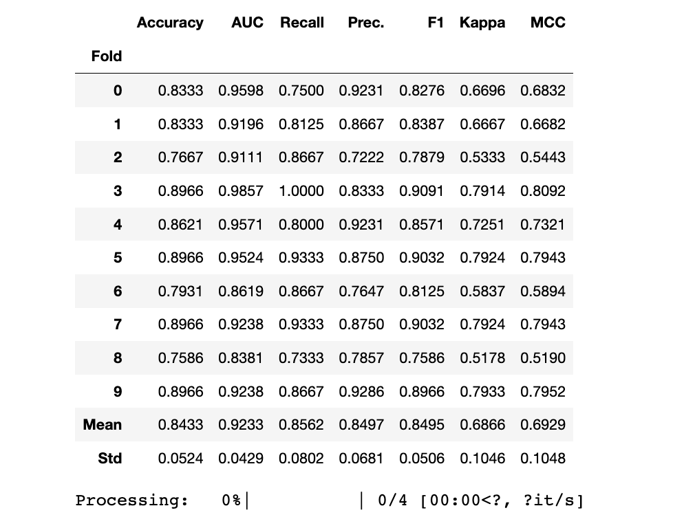
LightGBM
print("LGBM Model")
lgb_clf = create_model("lightgbm")
lgb_clf_scoregrid = pull()
LGBM Model
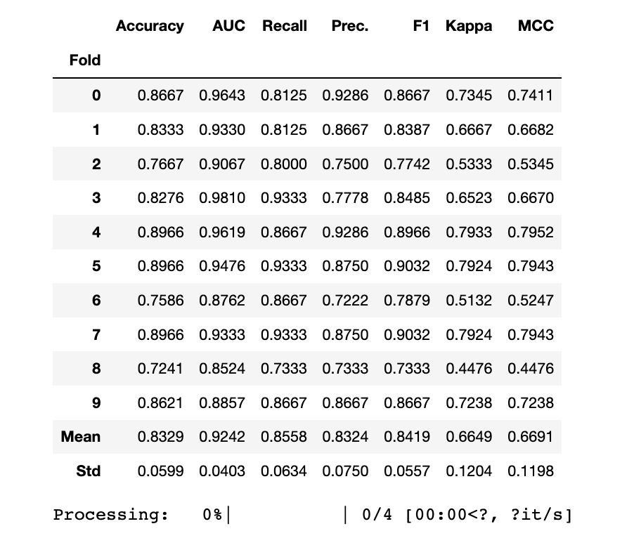
GBC
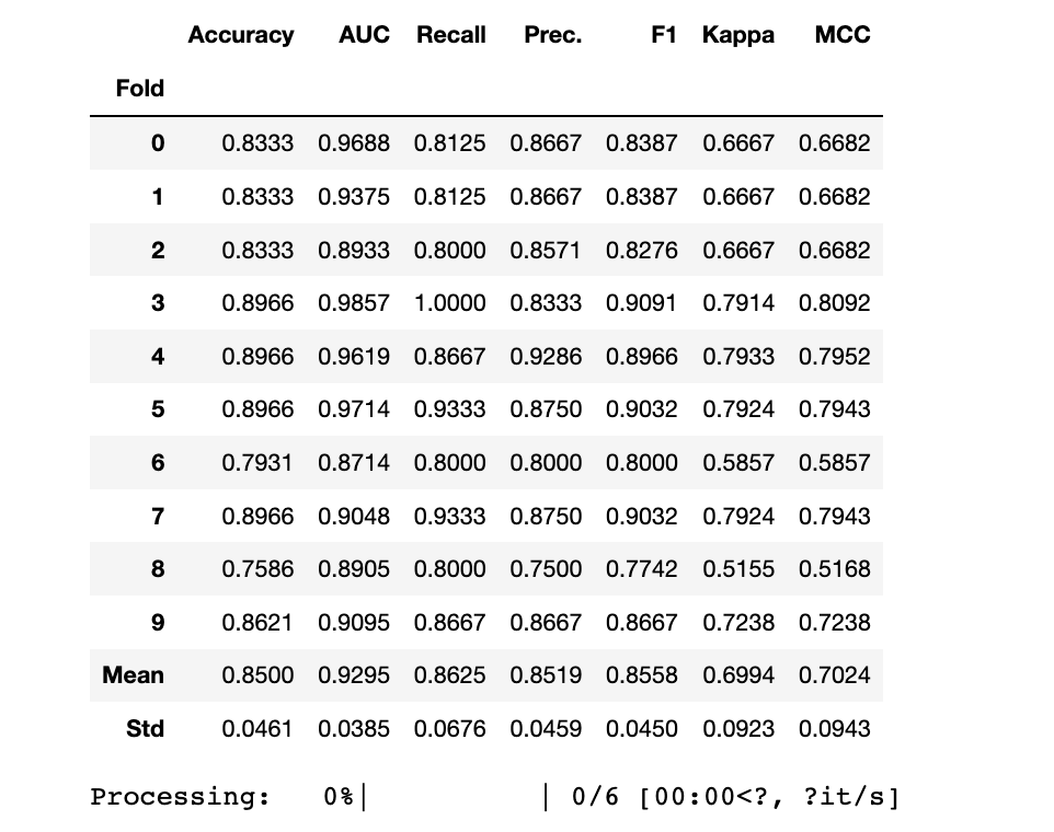
print("GBC Model")
gbc_clf = create_model("gbc")
gbc_clf_scoregrid = pull()
GBC Model
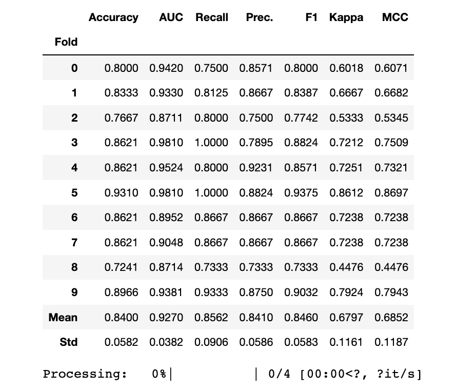
XGBoost
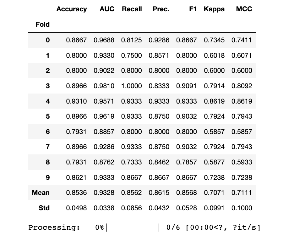
print("XGB Model")
xgb_clf = create_model("xgboost")
xgb_clf_scoregrid = pull()
XGB Model
7 使用Pycaret进行超参数调优
7.1 模型调优
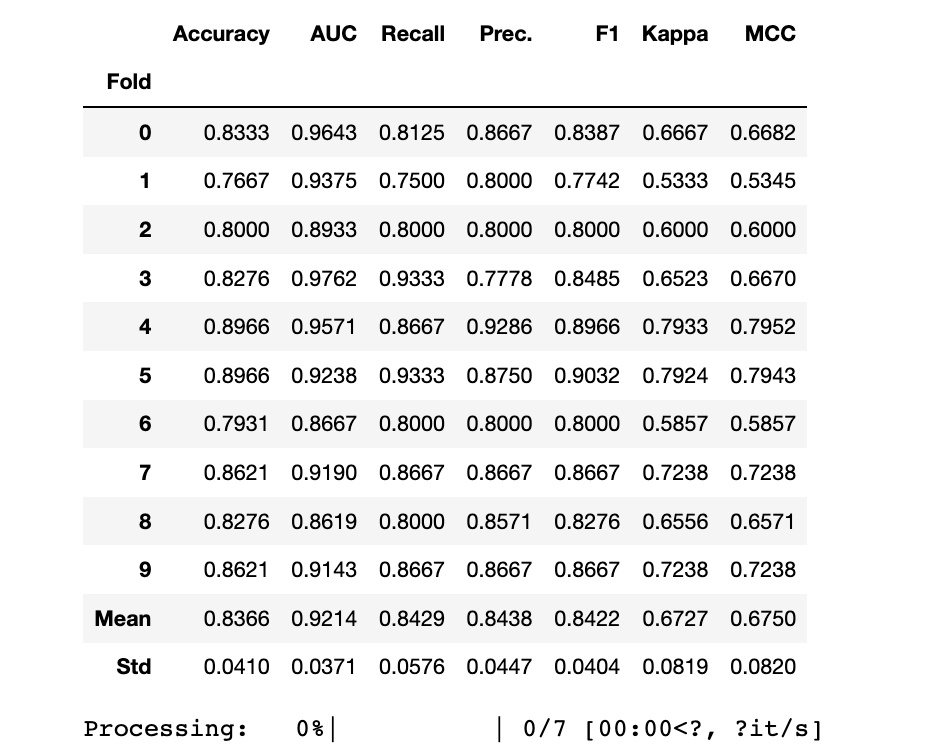
LightGBM
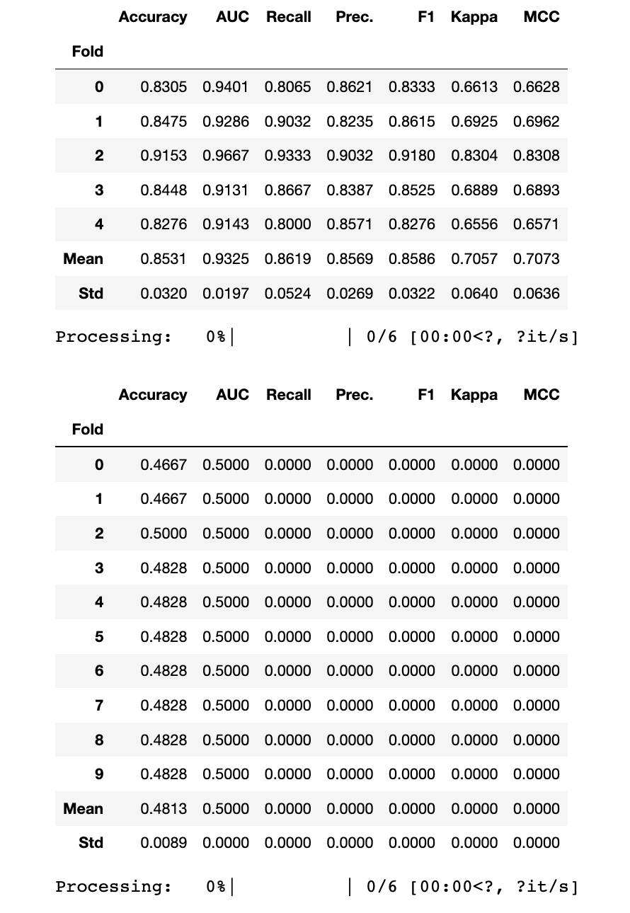
print("Before Tuning")
print(lgb_clf_scoregrid.loc[["Mean","Std"]])
print("")
lgb_clf = tune_model(lgb_clf,choose_better=True)
print(lgb_clf)
Before Tuning  Accuracy     AUC  Recall   Prec.      F1   Kappa     MCC
Fold
Mean    0.8433  0.9233  0.8562  0.8497  0.8495  0.6866  0.6929
Std     0.0524  0.0429  0.0802  0.0681  0.0506  0.1046  0.1048
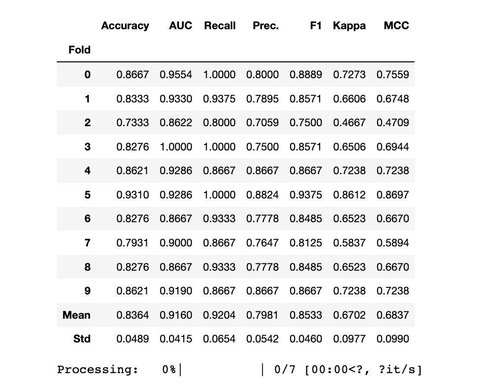
GBC
print("Before Tuning")
print(gbc_clf_scoregrid.loc[["Mean","Std"]])
print("")
gbc_clf = tune_model(gbc_clf,choose_better=True)
print(gbc_clf)
Before Tuning  Accuracy     AUC  Recall   Prec.      F1   Kappa     MCC
Fold
Mean    0.8329  0.9242  0.8558  0.8324  0.8419  0.6649  0.6691
Std     0.0599  0.0403  0.0634  0.0750  0.0557  0.1204  0.1198
XGBoost
print("Before Tuning")
print(xgb_clf_scoregrid.loc[["Mean","Std"]])
print("")
xgb_clf = tune_model(xgb_clf,choose_better = True)
print(xgb_clf)
Before Tuning  Accuracy     AUC  Recall   Prec.      F1   Kappa     MCC
Fold
Mean    0.8400  0.9270  0.8562  0.8410  0.8460  0.6797  0.6852
Std     0.0582  0.0382  0.0906  0.0586  0.0583  0.1161  0.1187
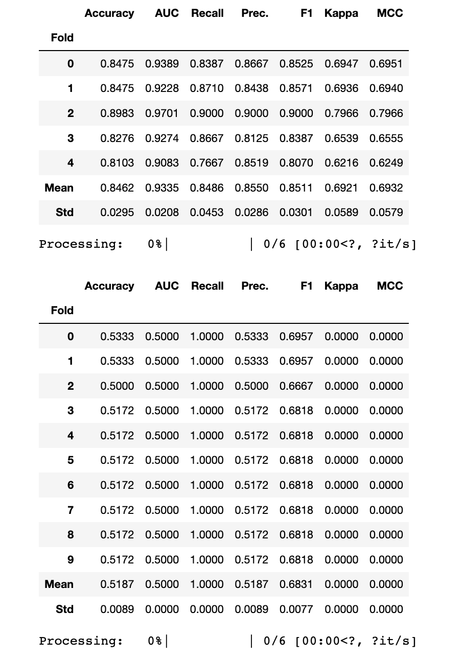
7.2 模型集成
-
Bagged & Boosting 方法
-
Blending
-
Stacking
LightGBM
# Original
print(lgb_clf_scoregrid.loc[['Mean', 'Std']])  # Compare the original against bagged and boosted  # Bagged
lgb_clf = ensemble_model(lgb_clf,fold =5,choose_better = True)
# Boosted
lgb_clf = ensemble_model(lgb_clf,method="Boosting",choose_better = True)
      Accuracy     AUC  Recall   Prec.      F1   Kappa     MCC
Fold
Mean    0.8433  0.9233  0.8562  0.8497  0.8495  0.6866  0.6929
Std     0.0524  0.0429  0.0802  0.0681  0.0506  0.1046  0.1048
GBC
# Original
print(gbc_clf_scoregrid.loc[['Mean', 'Std']])  # Compare the original against bagged and boosted  # Bagged
gbc_clf = ensemble_model(gbc_clf,fold =5,choose_better = True)
# Boosted
gbc_clf = ensemble_model(gbc_clf,method="Boosting",choose_better = True)
      Accuracy     AUC  Recall   Prec.      F1   Kappa     MCC
Fold
Mean    0.8329  0.9242  0.8558  0.8324  0.8419  0.6649  0.6691
Std     0.0599  0.0403  0.0634  0.0750  0.0557  0.1204  0.1198
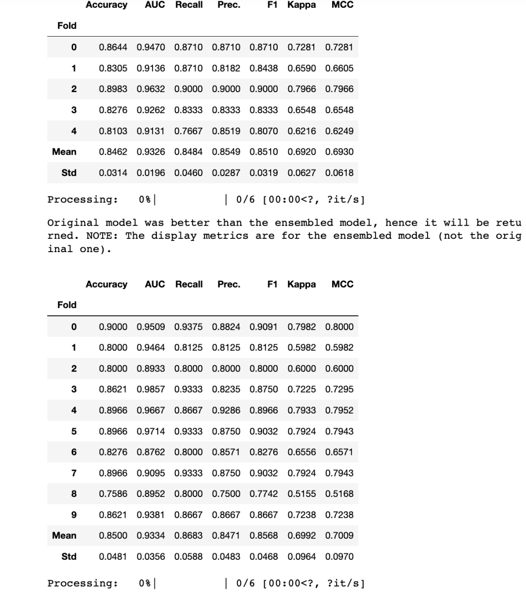
XGBoost
# Original
print(xgb_clf_scoregrid.loc[['Mean', 'Std']])  # Compare the original and boosted against bagged and boosted  # Bagged
xgb_clf = ensemble_model(xgb_clf,fold =5,choose_better = True)
# Boosted
xgb_clf = ensemble_model(xgb_clf,method="Boosting",choose_better = True)
      Accuracy     AUC  Recall   Prec.      F1   Kappa     MCC
Fold
Mean    0.8400  0.9270  0.8562  0.8410  0.8460  0.6797  0.6852
Std     0.0582  0.0382  0.0906  0.0586  0.0583  0.1161  0.1187
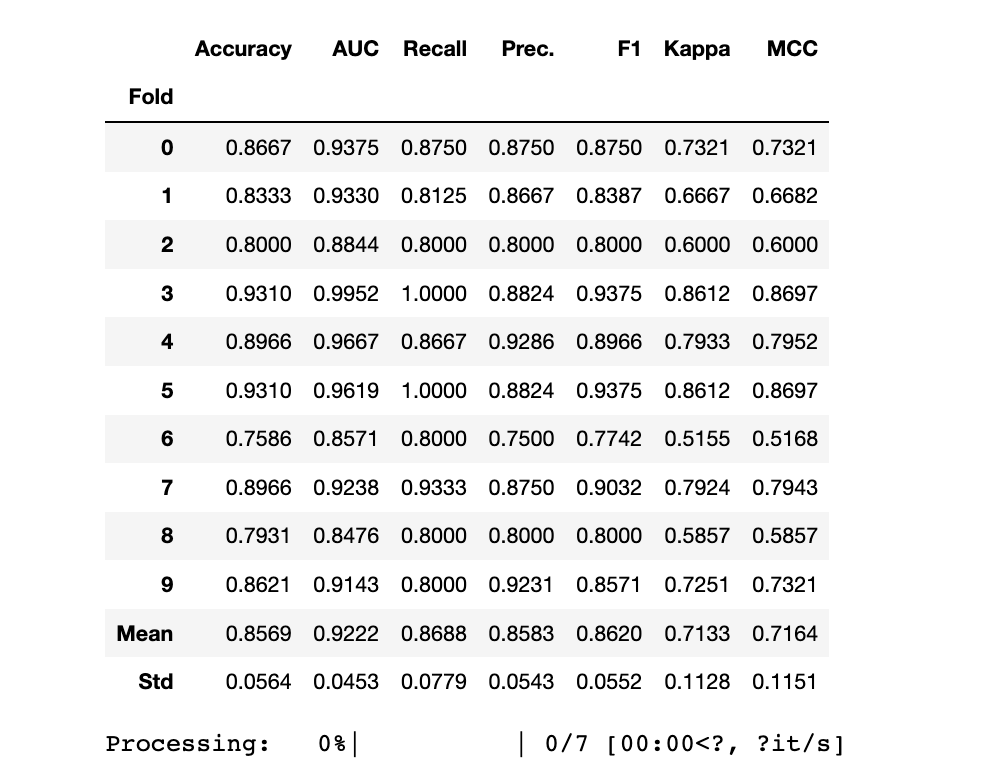
7.3.1 Blend Models
blend_models([lgb_clf, gbc_clf, xgb_clf],choose_better=True)
7.3.2 Stacking
stacker = stack_models(lgb_clf,gbc_clf) #remove xgb as some issues
print(stacker)
8 模型评估
# evaluate_model(lgb_clf)
# evaluate_model(gbc_clf)
# evaluate_model(xgb_clf)
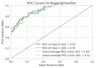
8.1 ROC-AUC
plot_model(stacker, plot = 'auc')
# Stacked classifier from ensembling
plot_model(lgb_clf, plot = 'auc')
# lgb最适合Bagging集成并被选中
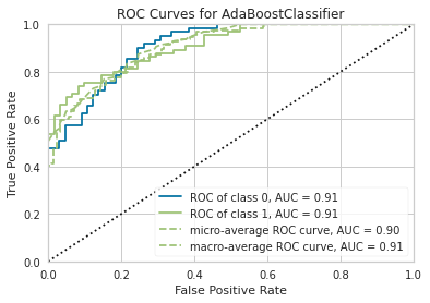
plot_model(gbc_clf, plot = 'auc')
# gbc最适合Boosting集成并被选中
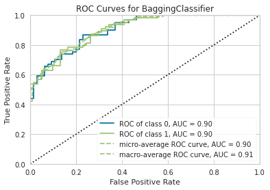
plot_model(xgb_clf, plot = 'auc')
# 基本的xgb分类器在经过调优和集成后仍然表现最好,因此选择了它 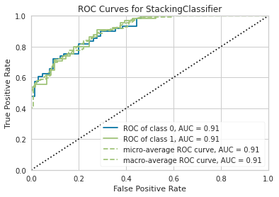
8.2 混淆矩阵
plot_model(stacker,   plot = 'confusion_matrix',   plot_kwargs = {'percent' : True})
plot_model(lgb_clf,   plot = 'confusion_matrix',   plot_kwargs = {'percent' : True})
plot_model(gbc_clf,   plot = 'confusion_matrix',   plot_kwargs = {'percent' : True})
plot_model(xgb_clf, plot = 'confusion_matrix', plot_kwargs = {'percent' : True}) 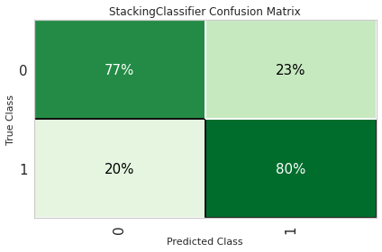


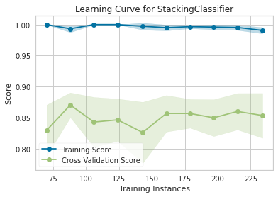
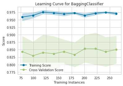
8.3 学习曲线
plot_model(stacker, plot = 'learning')
plot_model(lgb_clf, plot = 'learning')
就到这里了!
这篇关于企业级实战项目:基于 pycaret 自动化预测公司是否破产的文章就介绍到这儿,希望我们推荐的文章对编程师们有所帮助!


