轻知识库︱apple.Turicreate数据结构SGraph以及关系网络SNA分析（三）

本文主要是介绍轻知识库︱apple.Turicreate数据结构SGraph以及关系网络SNA分析（三），希望对大家解决编程问题提供一定的参考价值，需要的开发者们随着小编来一起学习吧！

笔者之前在学SNA时候对这块内容基本了解，这次遇到了apple.Turicreate，觉得该库可以通用性很强，而且算法面很多。本篇结构先来看看：

1、SGraph

2、关系网络的点出度、点入度、点密度、特征向量中心度

—- 点出度

—- 点入度

—- 点密度（triangle_counting）

—- 特征向量中心度（pagerank）

3、关系网络分析——社群发现

—- 标签概率社群发现算法, 有监督学习任务 ，用于监督性分类模型

—- K-core分解模型， 无监督学习任务 ，用于聚类

4、图论算法

—- 1.Single-source shortest path 最短路径

—- 2.连通分支（Connected Component）

—- 3.Graph coloring 图的最大独立集（最大团问题）

.

---

一、数据格式SGraph

数据结构SGraph
专业的图结构数据结构,看到的第一个这么正式的。 可扩展的图形数据结构。 SGraph数据结构允许在顶点和边上使用任意字典属性，提供灵活的顶点和边界查询功能，以及与SFrame之间的无缝转换。
官网链接：https://apple.github.io/turicreate/docs/api/generated/turicreate.SGraph.html#turicreate.SGraph

1.基本元素

SGraph(vertices=None, edges=None, vid_field='__id', src_field='__src_id', dst_field='__dst_id')

三大基本元素:

• vid_field:顶点
• src_field:原点
• dst_field:终点

由此构成两个重要概念：

• vertex,顶点
• edges,边线

vertex以及edges是贯穿SGraph以及图分析的两大元素。
.

2.如何创建SGraph

• 第一种是累加的方式，先创建一个空白的SGraph

from turicreate import SGraph, Vertex, Edge
g = SGraph()
verts = [Vertex(0, attr={'breed': 'labrador'}),Vertex(1, attr={'breed': 'labrador'}),Vertex(2, attr={'breed': 'vizsla'})]
g = g.add_vertices(verts)
g = g.add_edges(Edge(1, 2))

• 第二种方式比第一种更简洁：

g = SGraph().add_vertices([Vertex(i) for i in range(10)]).add_edges([Edge(i, i+1) for i in range(9)])
g.edges

• 第三种，从SFrame格式转换为SGraph

from turicreate import SFrame
url = 'https://static.turi.com/datasets/bond/bond_edges.csv'
edge_data = SFrame.read_csv(url)
print(edge_data)g = SGraph()
g = g.add_edges(edge_data, src_field='src', dst_field='dst')
print g

重要案例：简易版知识图谱——将顶点、边缘信息一起加载入SGraph

# 顶点信息
url = 'https://static.turi.com/datasets/bond/bond_vertices.csv'
vertex_data = SFrame.read_csv(url)
# 边缘信息
url = 'https://static.turi.com/datasets/bond/bond_edges.csv'
edge_data = SFrame.read_csv(url)print(vertex_data)
print(edge_data)g = SGraph(vertices=SFrame(vertex_data_frame), edges=edge_data, vid_field='name',src_field='src', dst_field='dst')

看看数据结构：

上面是顶点信息表，name就是顶点的名字，而其中三个字段，gender,license_to_kill,villian三个指标就是顶点信息。
下面一张表是边缘信息表，src起始点，dst终点，relation是两者的关系。
这样顶点、边缘信息就可以保存一些自己的信息内容，有一点知识图谱的味道了。
.

3.SGraph的保存与读入

# 图结构的读入与保存
g.save('james_bond.sgraph')
new_graph = turicreate.load_sgraph('james_bond.sgraph')

.

4.提取顶点、边缘信息

# 查询顶点信息
sub_verts = g.get_vertices(ids=['James Bond'])
print sub_verts
print g.vertices# 查询边缘信息
sub_edges = g.get_edges(fields={'relation': 'worksfor'})
print sub_edges
print g.edges

基本两种方式：g.get_vertices() 以及g.vertices
前者可以g.get_vertices() 定位到个人，而后面一个是返回全部信息。
.

5.顶点、边缘信息修改

g.edges['relation'] = g.edges['relation'].apply(lambda x: x[0].upper())
g.get_edges().print_rows(5)

g.edges[‘relation’]就可以定位到边缘信息中的relation字段，然后就可以跟dataframe一样进行赋值与修改。
如果要新加边缘或顶点信息，跟dataframe一样，可以这样赋值:

# 额外新加标注内容g.edges['weight'] = 1.0
del g.edges['weight']

可用于后续建模，weight的使用
.

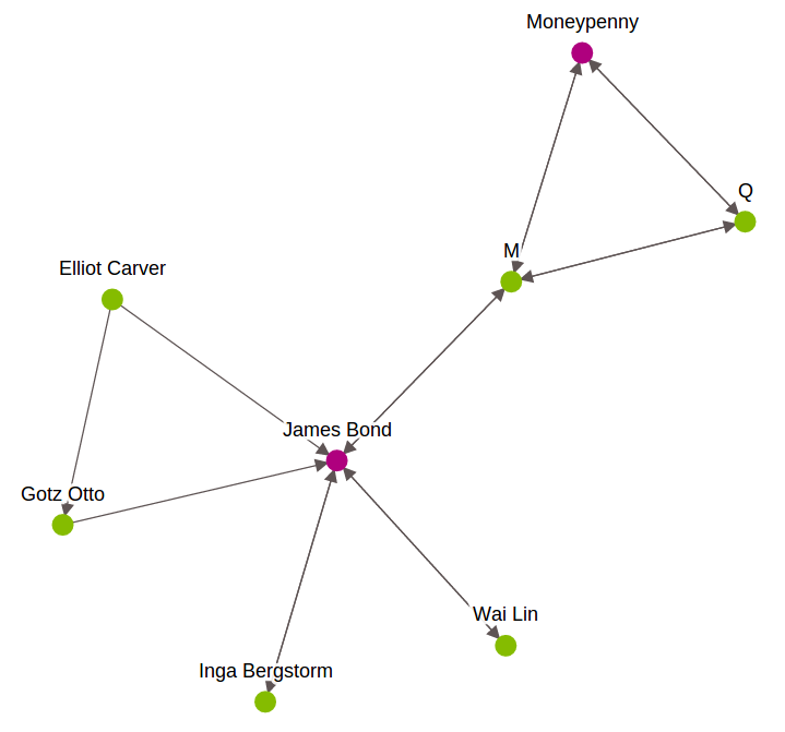
6.查找近邻子集

targets = ['James Bond', 'Moneypenny']
subgraph = g.get_neighborhood(ids=targets, radius=1, full_subgraph=True)
subgraph
# radius 代表辐射半径
# full_subgraph = True,代表近邻点之间的边是否全部涵盖，True代表即使跟AB没有关系，也需要全部加上

full_subgraph 这个参数，如下图的Elliot Carver 与otz Otto之间的边缘线，跟主查询的内容无关，也需要一起找出，比较全面，都为True比较好。

.

---

二、关系网络的点出度、点入度、点密度、特征向量中心度（pagerank）

SNA笔者是在R语言之前有学过一阵子，需要看的可以去看看之前写的博客：
R语言︱SNA-社会关系网络 R语言实现专题（基础篇）（一）
R语言︱SNA-社会关系网络—igraph包（中心度、中心势）（二）
R语言︱SNA-社会关系网络—igraph包（社群划分、画图）（三）
在apple.Turicreate中的官方链接：https://apple.github.io/turicreate/docs/userguide/graph_analytics/intro.html

来稍微回顾一下关系网络点入度、点出度的大致结构。

.

1.点度中心度——triple_apply()

'''
triple_apply可以同时执行三样内容
总点度 = 点入度 + 点出度
'''
def increment_degree(src, edge, dst):src['degree'] += 1dst['degree'] += 1return (src, edge, dst)
g.vertices['degree'] = 0g = g.triple_apply(increment_degree, mutated_fields=['degree'])
print g.vertices.sort('degree', ascending=False)  

triple_apply是可以输入三个图元素并进行计算的函数，比较灵活。

从结果看到，deree就是每个顶点的总点度
.

2.点入度、点出度

# 数据加载
from turicreate import SFrame, SGraph
url = 'https://static.turi.com/datasets/bond/bond_edges.csv'
data = SFrame.read_csv(url)
g = SGraph().add_edges(data, src_field='src', dst_field='dst')# 计算点入度 以及 点出度
from turicreate import degree_counting
deg = degree_counting.create(g)
deg_graph = deg.graph # a new SGraph with degree data attached to each vertex
deg_graph.vertices    # 图谱顶点，点出点入总表
in_degree = deg_graph.vertices[['__id', 'in_degree']]
out_degree = deg_graph.vertices[['__id', 'out_degree']]
print(in_degree)
print(out_degree)

degree_counting启动计算图计数函数，in_degree以及out_degree就是点入度以及点出度。

同时可以将点度、点入度以及点出度都放在顶点信息表之中：

g.vertices['in_degree'] = in_degree['in_degree']
g.vertices['out_degree'] = out_degree['out_degree']
g.vertices

.

3.pagerank——特征向量中心度

pr = turicreate.pagerank.create(g, max_iterations=10)
print(pr.summary())

其中启动之后可以查询一下一些属性：

# 可查询属性
pr.training_time      # 训练时间
pr.graph              # 图数据
pr.reset_probability  # 随机转移概率
pr.pagerank           # 顶点的pagerank值
pr.num_iterations     # 迭代次数
pr.threshold          # L1规范的阈值
max_iterations        # 最大迭代次数

来看看最高的pagerank值的方式：

# pagerank最高的top10
print(pr.pagerank.topk('pagerank', k=10))

.

4.顶点近邻密度的指标——triangle_counting

衡量顶点近邻密度的指标，越高密度越大，价值越大。

tri = turicreate.triangle_counting.create(sg)

一些属性值。

print(tri.summary())
tri.num_triangles # tri的三角总数
tri.training_time  # 训练时间
tri.triangle_count # 三角计数表 核心，跟pagerank一致
tri.triangle_count.topk('triangle_count', k=10)  # 排名前10的三角数

跟点度还是挺像的，也跟pagerank一样，作为分析的一种指标。来看：

.

---

三、关系网络分析——社群发现

这里会介绍基于标签概率社群发现算法和K-core分解模型。在turicreate之中，两个算法有以下两个关键的擅长之处:

• 标签概率社群发现算法, 有监督学习任务 ，用于监督性分类模型
• K-core分解模型， 无监督学习任务 ，用于聚类
  .

1.LabelPropagationModel 基于标签概率社群发现算法

来源网址

主函数：

turicreate.label_propagation.create(graph, label_field, threshold=0.001, weight_field='', self_weight=1.0, undirected=False, max_iterations=None, _single_precision=False, _distributed='auto', verbose=True)

训练与预测的数据集都可以放在一块儿：

id label001 0002 1003 None... ...

如果是需要预测的样本，可以用None的形式,放在数据集之中，然后通过模型训练，其会自动给出label（g.labels）

来一则案例：

# 加载数据
g = turicreate.load_graph('http://snap.stanford.edu/data/email-Enron.txt.gz',format='snap')# 随机生成标签列，label
import random
def init_label(vid):x = random.random()if x < 0.2:return 0elif x > 0.9:return 1elif (x > 0.3 )&( x < 0.5):return 2else:return None
g.vertices['label'] = g.vertices['__id'].apply(init_label, int)# 查看训练样式
g.vertices.print_rows(num_rows=100, num_columns=2)# label_propagation建模
m = turicreate.label_propagation.create(g, label_field='label')

数据长这样：

其中模型就保存在m之中。模型之中存储的一些属性值有：

labels = m.labels 
print(m.self_weight)
print(m.weight_field)
print(m.label_field)
print(m.undirected)

其中m.labels 就是主要输出内容，可见：

可以观察到，对于label = none的其也会给出概率预测的情况。跟普通的机器学习是一样一样的。
所以，该内容可以跟ML一样，作为有监督训练的一种方式。
.

2、K-core decomposition k-core分解

Kitsak等人[1]第一次系统分析了这个问题。他们指出度和介数往往不能很精确描述一个节点的传播能力，而利用k-core分解，一个节点的核数更好刻画了节点的传播能力。
有点像层次聚类，一步一步删除附近的劣质线条。
理论地址，相关paper

主函数：

create(graph, kmin=0, kmax=10, verbose=True)

K值越高，网络越核心，k-core值越大表明子网络越处于核心的地位

g = turicreate.load_graph('http://snap.stanford.edu/data/email-Enron.txt.gz', format='snap')
kc = turicreate.kcore.create(g,kmax = 20)
# 在g中赋值
g.vertices['core_id'] = kc.graph.vertices['core_id']print(kc.core_id)   # 聚类之后的每个ID的表格
#kc.graph
#kc.kmax

如果指定了Kmax为20，就像聚类一样，会给每个ID一个标签值，可见：

.

---

四、图论算法

1.Single-source shortest path 最短路径

The single-source shortest path problem is to find the shortest path from all vertices in the graph to a user-specified target node.

主函数：

create(graph, source_vid, weight_field="", max_distance=1e30, verbose=True)

参数解释：
weight_field : string, optional,The edge field representing the edge weights. If empty, uses unit weights.
verbose : bool, optional,If True, print progress updates.

看看一个案例：从Microsoft 到 Weyerhaeuser 的最短路径是什么。

sssp = turicreate.shortest_path.create(sg, source_vid='Microsoft')
sssp.get_path(vid='Weyerhaeuser',highlight=['Microsoft', 'Weyerhaeuser']) sssp.distance # 每个从microsoft出发的，顶点距离分布表
sssp.distance.topk('distance', k=10)

老版本中get_path，有下面两个参数：arrows=True, ewidth=1.5 ，现在的版本已经没有了。
返回结果：

[('Microsoft', 0.0),('Google', 1.0),('Tax avoidance', 2.0),('Weyerhaeuser', 3.0)]

.

2.连通分支（Connected Component）

官方链接

在一个图中，某个子图的任意两点有边连接，并且该子图去剩下的任何点都没有边相连。
1 Compute the number of weakly connected components in the graph.
2 Return a model object with total number of weakly connected components as well as the component ID for each vertex in the graph.
3 A weakly connected component is a maximal set of vertices such that there exists an undirected path between any two vertices in the set.
4 从大网络中抽取出密集型网络，网络中每个顶点都会两两互相连接

g = turicreate.load_graph('http://snap.stanford.edu/data/email-Enron.txt.gz', format='snap')
cc = turicreate.connected_components.create(g)
cc.summary()
cc.component_id  # 顶点ID
cc.graph.edges

返回的是一个SGraph图谱。该SGraph就是完整的Connected Components
.

3.Graph coloring 图的最大独立集（最大团问题）

• Compute the graph coloring. Assign a color to each vertex such that
  no adjacent vertices have the same color.
• Return a model object with total number of colors used as well as the
  color ID for each vertex in the graph.
• This algorithm is greedy and is not guaranteed to find the minimum
  graph coloring. It is also not deterministic, so successive runs may
  return different answers.
• 使用贪心算法,而且结果具有随机性，按照某种规则对一个图的每个顶点或者边分配一个颜色(编号)，称为对图的着色。能按此规则完成着色的最小颜色数称为色数(chromatic
  number)，记为χ(G)。
  参考博客：http://blog.51cto.com/nxlhero/1213947

from turicreate import graph_coloring
color = graph_coloring.create(g)print(color.color_id)
print(color.num_colors)

查看一下每个ID的颜色ID。

---

公众号“素质云笔记”定期更新博客内容：

这篇关于轻知识库︱apple.Turicreate数据结构SGraph以及关系网络SNA分析（三）的文章就介绍到这儿，希望我们推荐的文章对编程师们有所帮助！

---