因果推断笔记——因果图建模之Uber开源的CausalML（十二）

本文主要是介绍因果推断笔记——因果图建模之Uber开源的CausalML（十二），希望对大家解决编程问题提供一定的参考价值，需要的开发者们随着小编来一起学习吧！

它提供了一个标准框架，允许用户从实验或观察数据估计条件平均治疗效果(CATE)或个人治疗效果(ITE)。本质上，它估计了干预T对具有观察到的特征X的用户结果Y的因果影响，而没有对模型形式有很强的假设。

github：https://github.com/uber/causalml

其余两篇开源项目的文章：
因果推断笔记——因果图建模之微软开源的EconML（五）
因果推断笔记——因果图建模之微软开源的dowhy（一）

---

---

1 CausalML 、 EconML、dowhy异同

相比拉私活，causalML主要是面向Uplift 的模型，econML更加全面一些。

1.1 econML 主要估计器

主要的Estimation Methods估计器：

• Double Machine Learning (aka RLearner)
• Dynamic Double Machine Learning
• Causal Forests
• Orthogonal Random Forests
• Meta-Learners
• Doubly Robust Learners
• Orthogonal Instrumental Variables
• Deep Instrumental Variables

Interpretability解释性方面：

• Tree Interpreter of the CATE model
• Policy Interpreter of the CATE model
• SHAP values for the CATE model

Causal Model Selection and Cross-Validation 模型选择方面：

• Causal model selection with the RScorer
• First Stage Model Selection

1.2 CausalML 主要的估计器

• Tree-based algorithms

  • Uplift tree/random forests on KL divergence, Euclidean Distance, and Chi-Square [1]
  • Uplift tree/random forests on Contextual Treatment Selection [2]
  • Causal Tree [3] - Work-in-progress

• Meta-learner algorithms

  • S-learner [4]
  • T-learner [4]
  • X-learner [4]
  • R-learner [5]
  • Doubly Robust (DR) learner [6]
  • TMLE learner [7]

• Instrumental variables algorithms

  • 2-Stage Least Squares (2SLS)
  • Doubly Robust (DR) IV [8]

• Neural-network-based algorithms

  • CEVAE [9]
  • DragonNet [10] - with causalml[tf] installation (see Installation)

1.3 dowhy的估计器

使用统计方法对表达式进行估计，识别之后的估计

• 「基于估计干预分配的方法」
  • 基于倾向的分层（Propensity-based Stratification）
  • 倾向得分匹配（Propensity Score Matching）
  • 逆向倾向加权（Inverse Propensity Weighting）
• 「基于估计结果模型的方法」
  • 线性回归（Linear Regression）
  • 广义线性模型（Generalized Linear Models）
• 「基于工具变量等式的方法」
  • 二元工具/Wald 估计器（Binary Instrument/Wald Estimator）
  • 两阶段最小二乘法（Two-stage least squares）
  • 非连续回归（Regression discontinuity）
• 「基于前门准则和一般中介的方法」
  • 两层线性回归（Two-stage linear regression）

1.3 简单对比：dowhy \ causalml\ econml

可以看到econML比较全面，涵盖了DML、uplift model、IV、Doubly Robust等
dowhy比较基础，涵盖的的是psm、psm、psw、iv等，
causalML主要集中在uplift model，S-learner 、 T-learner、X-learner、DR等,Tree-based 算是多出的，还有几款NN-Based的

同样，解释性，econml / causalml款都有，涵盖shap / Tree Interpreter /Policy Interpreter

---

2 安装

window10 倒腾了大半天，各种报错。。问题会围绕Microsoft visual c++14.0、MicrosoftVisualStudio 等，还有要安装tf会有些问题；还有Built的时候会有一些报错。。
整体使用起来，方便性不如econml，后面还会有一些报错。
所以没深究就放弃了，还是用云服务器比较省心：

$ git clone https://github.com/uber/causalml.git
$ cd causalml
$ pip install -r requirements.txt
$ pip install causalml

---

3 Quick Start

3.1 S, T, X, and R Learners估计ATE

这里有一个 问题，就是xgboost.XGBRegressor，在causalml默认是xgboost = 1.4.2版本的，但是这个版本会出现报错：

AttributeError: type object 'cupy.core.core.broadcast' has no attribute '__reduce_cython__'

也就是这里需要注意，如果是cpu调用，需要Predictor = 'cpu_predictor'，但是，好像causalML封装的有些问题，from causalml.inference.meta import XGBTRegressor，所以一直会报上面的错，只能回退xgboost版本到1.3.1就正常了。

20211213更新一个神奇的bug
xgboost.XGBClassifier( predictor = ‘cpu_predictor’) ，在1.3.1 版本下，第一次运行可以正常，第二次再次model.fit()的时候，还是会出现'__reduce_cython__'，
笔者经过多轮尝试，回退到1.2.1，终于恢复正常
奇怪的是，1.3.1版本下，xgboost.XGBRegressor 多轮运行是正常的，具体原因未知… 且在其他window系统下，XGBClassifier在1.3.3 也是正常的，非常奇怪。。

from causalml.inference.meta import LRSRegressor
from causalml.inference.meta import XGBTRegressor, MLPTRegressor
from causalml.inference.meta import BaseXRegressor
from causalml.inference.meta import BaseRRegressor
from xgboost import XGBRegressor
from causalml.dataset import synthetic_datay, X, treatment, _, _, e = synthetic_data(mode=1, n=1000, p=5, sigma=1.0)lr = LRSRegressor()
te, lb, ub = lr.estimate_ate(X, treatment, y)
print('Average Treatment Effect (Linear Regression): {:.2f} ({:.2f}, {:.2f})'.format(te[0], lb[0], ub[0]))xg = XGBTRegressor(random_state=42)
te, lb, ub = xg.estimate_ate(X, treatment, y)
print('Average Treatment Effect (XGBoost): {:.2f} ({:.2f}, {:.2f})'.format(te[0], lb[0], ub[0]))nn = MLPTRegressor(hidden_layer_sizes=(10, 10),learning_rate_init=.1,early_stopping=True,random_state=42)
te, lb, ub = nn.estimate_ate(X, treatment, y)
print('Average Treatment Effect (Neural Network (MLP)): {:.2f} ({:.2f}, {:.2f})'.format(te[0], lb[0], ub[0]))xl = BaseXRegressor(learner=XGBRegressor(random_state=42))
te, lb, ub = xl.estimate_ate(X, treatment, y, e)
print('Average Treatment Effect (BaseXRegressor using XGBoost): {:.2f} ({:.2f}, {:.2f})'.format(te[0], lb[0], ub[0]))rl = BaseRRegressor(learner=XGBRegressor(random_state=42))
te, lb, ub =  rl.estimate_ate(X=X, p=e, treatment=treatment, y=y)
print('Average Treatment Effect (BaseRRegressor using XGBoost): {:.2f} ({:.2f}, {:.2f})'.format(te[0], lb[0], ub[0]))

这里 y - 因变量, X-协变量, treatment-干预, e - PS倾向性得分

这里对应使用的估计器是：

• LRSRegressor —— Linear Regression
• XGBTRegressor—— XGBoost
• MLPTRegressor—— Neural Network (MLP)
• BaseXRegressor—— BaseXRegressor using XGBoost
• BaseRRegressor—— BaseRRegressor using XGBoost

输出的结果，$te,lb,ub$，代表，$ATE$总体效应，以及置信区间$[lb,ub]$

3.2 meta元学习估计ATE/ITE

这里参考官方文档：meta_learners_with_synthetic_data.ipynb
当然，这里注意到该教程中干预是0/1二分类的，那么后面有一份类似的教程是，干预可以是multiple_treatment所以可参考：meta_learners_with_synthetic_data_multiple_treatment.ipynb

import pandas as pd
import numpy as np
from matplotlib import pyplot as plt
from sklearn.linear_model import LinearRegression
from sklearn.model_selection import train_test_split
import statsmodels.api as sm
from xgboost import XGBRegressor
import warningsfrom causalml.inference.meta import LRSRegressor
from causalml.inference.meta import XGBTRegressor, MLPTRegressor
from causalml.inference.meta import BaseXRegressor, BaseRRegressor, BaseSRegressor, BaseTRegressor
from causalml.match import NearestNeighborMatch, MatchOptimizer, create_table_one
from causalml.propensity import ElasticNetPropensityModel
from causalml.dataset import *
from causalml.metrics import *warnings.filterwarnings('ignore')
plt.style.use('fivethirtyeight')%matplotlib inlineimport causalml
print(causalml.__version__)

生成数据：

# Generate synthetic data using mode 1
y, X, treatment, tau, b, e = synthetic_data(mode=1, n=10000, p=8, sigma=1.0)

来看看众多的估计器：

3.2.1 『ATE』S-Learning 单模型 - 线性模型

S-Learner using LinearRegression

# Ready-to-use S-Learner using LinearRegression
learner_s = LRSRegressor()
ate_s = learner_s.estimate_ate(X=X, treatment=treatment, y=y)
print(ate_s)
print('ATE estimate: {:.03f}'.format(ate_s[0][0]))
print('ATE lower bound: {:.03f}'.format(ate_s[1][0]))
print('ATE upper bound: {:.03f}'.format(ate_s[2][0]))

输出ATE:

(array([0.68844541]), array([0.64017928]), array([0.73671154]))
ATE estimate: 0.688
ATE lower bound: 0.640
ATE upper bound: 0.737

3.2.2 『ATE』双模型T-Learner + XGB回归

# Ready-to-use T-Learner using XGB
learner_t = XGBTRegressor()
ate_t = learner_t.estimate_ate(X=X, treatment=treatment, y=y)
print('Using the ready-to-use XGBTRegressor class')
print(ate_t)

输出：

Using the ready-to-use XGBTRegressor class
(array([0.53355931]), array([0.50912018]), array([0.55799843]))

3.2.3 『ATE』Base Learner 基础模型

# Calling the Base Learner class and feeding in XGB
learner_t = BaseTRegressor(learner=XGBRegressor())
ate_t = learner_t.estimate_ate(X=X, treatment=treatment, y=y)
print('\nUsing the BaseTRegressor class and using XGB (same result):')
print(ate_t)# Calling the Base Learner class and feeding in LinearRegression
learner_t = BaseTRegressor(learner=LinearRegression())
ate_t = learner_t.estimate_ate(X=X, treatment=treatment, y=y)
print('\nUsing the BaseTRegressor class and using Linear Regression (different result):')
print(ate_t)

有基础估计的，带上XGBRegressor回归 + LinearRegression线性模型
输出为：

Using the BaseTRegressor class and using XGB (same result):
(array([0.53355931]), array([0.50912018]), array([0.55799843]))Using the BaseTRegressor class and using Linear Regression (different result):
(array([0.68904064]), array([0.64912657]), array([0.7289547]))

3.2.4 『ATE』含/不含倾向得分的X-Learner + 基础模型

X Learner without propensity score input

# 前面两个是带倾向得分的# X Learner with propensity score input
# Calling the Base Learner class and feeding in XGB
learner_x = BaseXRegressor(learner=XGBRegressor())
ate_x = learner_x.estimate_ate(X=X, treatment=treatment, y=y, p=e)
print('Using the BaseXRegressor class and using XGB:')
print(ate_x)# Calling the Base Learner class and feeding in LinearRegression
learner_x = BaseXRegressor(learner=LinearRegression())
ate_x = learner_x.estimate_ate(X=X, treatment=treatment, y=y, p=e)
print('\nUsing the BaseXRegressor class and using Linear Regression:')
print(ate_x)# 后面两个是不带倾向得分的结果
# X Learner without propensity score input
# Calling the Base Learner class and feeding in XGB
learner_x = BaseXRegressor(XGBRegressor())
ate_x = learner_x.estimate_ate(X=X, treatment=treatment, y=y)
print('Using the BaseXRegressor class and using XGB without propensity score input:')
print(ate_x)# Calling the Base Learner class and feeding in LinearRegression
learner_x = BaseXRegressor(learner=LinearRegression())
ate_x = learner_x.estimate_ate(X=X, treatment=treatment, y=y)
print('\nUsing the BaseXRegressor class and using Linear Regression without propensity score input:')
print(ate_x)

输出为：

Using the BaseXRegressor class and using XGB:
(array([0.49851986]), array([0.47623108]), array([0.52080863]))Using the BaseXRegressor class and using Linear Regression:
(array([0.67178423]), array([0.63091207]), array([0.7126564]))

其中e是额外计算的倾向得分

3.2.5 『ATE』R Learner + 含/不含倾向得分

# R-Learnning 含倾向得分
# R Learner with propensity score input
# Calling the Base Learner class and feeding in XGB
learner_r = BaseRRegressor(learner=XGBRegressor())
ate_r = learner_r.estimate_ate(X=X, treatment=treatment, y=y, p=e)
print('Using the BaseRRegressor class and using XGB:')
print(ate_r)# Calling the Base Learner class and feeding in LinearRegression
learner_r = BaseRRegressor(learner=LinearRegression())
ate_r = learner_r.estimate_ate(X=X, treatment=treatment, y=y, p=e)
print('Using the BaseRRegressor class and using Linear Regression:')
print(ate_r)# R-Learnning 不含倾向得分
# R Learner without propensity score input
# Calling the Base Learner class and feeding in XGB
learner_r = BaseRRegressor(learner=XGBRegressor())
ate_r = learner_r.estimate_ate(X=X, treatment=treatment, y=y)
print('Using the BaseRRegressor class and using XGB without propensity score input:')
print(ate_r)# Calling the Base Learner class and feeding in LinearRegression
learner_r = BaseRRegressor(learner=LinearRegression())
ate_r = learner_r.estimate_ate(X=X, treatment=treatment, y=y)
print('Using the BaseRRegressor class and using Linear Regression without propensity score input:')
print(ate_r)

3.2.6 『ITE』S, T, X, R Learners求ITE/CATE

# S Learner
learner_s = LRSRegressor()
cate_s = learner_s.fit_predict(X=X, treatment=treatment, y=y)# T Learner
learner_t = BaseTRegressor(learner=XGBRegressor())
cate_t = learner_t.fit_predict(X=X, treatment=treatment, y=y)# X Learner with propensity score input
learner_x = BaseXRegressor(learner=XGBRegressor())
cate_x = learner_x.fit_predict(X=X, treatment=treatment, y=y, p=e)# X Learner without propensity score input
learner_x_no_p = BaseXRegressor(learner=XGBRegressor())
cate_x_no_p = learner_x_no_p.fit_predict(X=X, treatment=treatment, y=y)# R Learner with propensity score input 
learner_r = BaseRRegressor(learner=XGBRegressor())
cate_r = learner_r.fit_predict(X=X, treatment=treatment, y=y, p=e)# R Learner without propensity score input
learner_r_no_p = BaseRRegressor(learner=XGBRegressor())
cate_r_no_p = learner_r_no_p.fit_predict(X=X, treatment=treatment, y=y)

可以看到求总体的ATE不同ITE主要是，model.fit_predict 而不是model.estimate_ate

画图对比一下：

alpha=0.2
bins=30
plt.figure(figsize=(12,8))
plt.hist(cate_t, alpha=alpha, bins=bins, label='T Learner')
plt.hist(cate_x, alpha=alpha, bins=bins, label='X Learner')
plt.hist(cate_x_no_p, alpha=alpha, bins=bins, label='X Learner (no propensity score)')
plt.hist(cate_r, alpha=alpha, bins=bins, label='R Learner')
plt.hist(cate_r_no_p, alpha=alpha, bins=bins, label='R Learner (no propensity score)')
plt.vlines(cate_s[0], 0, plt.axes().get_ylim()[1], label='S Learner',linestyles='dotted', colors='green', linewidth=2)
plt.title('Distribution of CATE Predictions by Meta Learner')
plt.xlabel('Individual Treatment Effect (ITE/CATE)')
plt.ylabel('# of Samples')
_=plt.legend()

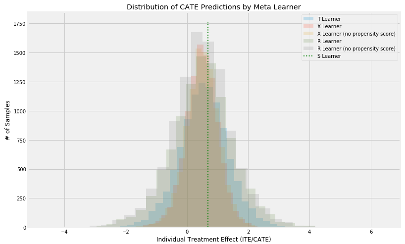
模型输出的分布，几个模型基本分布是一致的

3.3 Meta-Learner的评估精准性

3.3.1 MSE

Validating Meta-Learner Accuracy

train_summary, validation_summary = get_synthetic_summary_holdout(simulate_nuisance_and_easy_treatment,n=10000,valid_size=0.2,k=10)

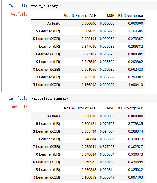
从结果可以对比差异还是蛮大的，还有KL Divergence散度指标,注意，simulate_nuisance_and_easy_treatment是一个模拟数据的函数，get_synthetic_summary_holdout模拟之后得到的结论，所以这个函数主要是在模拟运行。
如果有真实数据需要自己计算MSE / KL Divergence了。

按误差再来画一个各模型的对比图：

scatter_plot_summary_holdout(train_summary,validation_summary,k=10,label=['Train', 'Validation'],drop_learners=[],drop_cols=[])

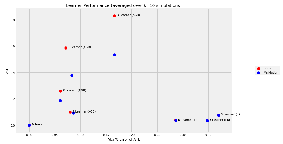
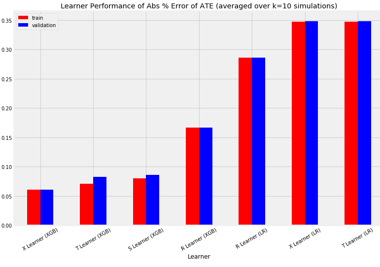
bar_plot_summary_holdout(train_summary,validation_summary,k=10,drop_learners=['S Learner (LR)'],drop_cols=[])

三个指标的柱状图，error of ATE / MSE / KL散度

3.3.2 AUUC

# Single simulation 生成数据
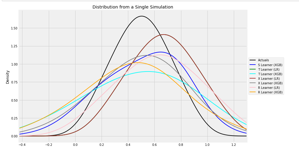
train_preds, valid_preds = get_synthetic_preds_holdout(simulate_nuisance_and_easy_treatment,n=50000,valid_size=0.2)#distribution plot for signle simulation of Training 查看数据分布
distr_plot_single_sim(train_preds, kind='kde', linewidth=2, bw_method=0.5,drop_learners=['S Learner (LR)',' S Learner (XGB)'])

其中来重点看一下get_synthetic_preds_holdout生成之后数据张什么样子，
因为生成过程比较慢，建议把n调小一些，其中train_preds是，涵盖了，元数据，倾向得分，各类模型的估计结果：

{'Actuals': array([0.79643095, 0.95486817, 0.76997445, ..., 0.75298567, 0.57918784,0.50598952]),'generated_data': {'y': array([2.82809532, 0.83627125, 2.96923917, ..., 3.69930311, 2.11858631,2.08442807]),'X': array([[0.80662423, 0.78623768, 0.55714673, 0.78484245, 0.7062874 ],[0.9777165 , 0.93201984, 0.94806163, 0.27111164, 0.91731333],[0.94459763, 0.59535128, 0.94004736, 0.78097312, 0.68469675],...,[0.9168486 , 0.58912275, 0.1413644 , 0.40006979, 0.21380953],[0.68509846, 0.47327722, 0.476474  , 0.5284623 , 0.7752548 ],[0.7854881 , 0.22649094, 0.79246468, 0.23035102, 0.46786142]]),'w': array([1, 0, 0, ..., 1, 1, 1]),'tau': array([0.79643095, 0.95486817, 0.76997445, ..., 0.75298567, 0.57918784,0.50598952]),'b': array([2.0569544 , 1.4065011 , 2.49147132, ..., 1.75627446, 1.76858932,1.16561357]),'e': array([0.9       , 0.27521434, 0.9       , ..., 0.9       , 0.85139268,0.53026066])},'S Learner (LR)': array([0.67412079, 0.67412079, 0.67412079, ..., 0.67412079, 0.67412079,0.67412079]),'S Learner (XGB)': array([0.71599877, 1.01481819, 0.45305347, ..., 1.33423424, 0.76635182,0.54931992]),'T Learner (LR)': array([1.02410448, 1.23423655, 0.98041236, ..., 0.96302446, 0.76681856,0.6616715 ]),'T Learner (XGB)': array([1.39729691, 2.1762352 , 0.18748665, ..., 1.81221414, 1.25306892,0.5382663 ]),'X Learner (LR)': array([1.02410448, 1.23423655, 0.98041236, ..., 0.96302446, 0.76681856,0.6616715 ]),'X Learner (XGB)': array([ 0.86962565,  2.17324671, -0.32896739, ...,  1.60033008,1.33514268,  0.41377797]),'R Learner (LR)': array([1.12468185, 1.35693603, 1.04248628, ..., 1.00324719, 0.75967883,0.57261269]),'R Learner (XGB)': array([0.49208722, 1.1459806 , 0.0804432 , ..., 1.74274731, 1.07263219,0.48373923])}

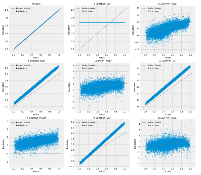
# Scatter Plots for a Single Simulation of Training Data
scatter_plot_single_sim(train_preds)

训练集的散点图：

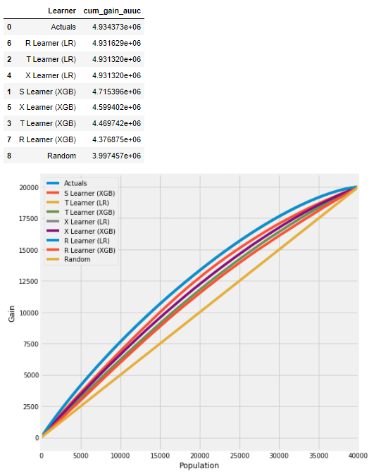
计算AUUC：

# Cumulative Gain AUUC values for a Single Simulation of Training Data
get_synthetic_auuc(train_preds, drop_learners=['S Learner (LR)'])

---

4 可解释性：Policy Learning Notebook

主要参考的是文档：binary_policy_learner_example.ipynb
另外一个更全面的在：uplift_tree_visualization.ipynb

import pandas as pd
import numpy as np
from matplotlib import pyplot as pltfrom sklearn.model_selection import cross_val_predict, KFold
from sklearn.ensemble import GradientBoostingRegressor, GradientBoostingClassifier
from sklearn.tree import DecisionTreeClassifierfrom causalml.optimize import PolicyLearner
from sklearn.tree import plot_tree
from lightgbm import LGBMRegressor
from causalml.inference.meta import BaseXRegressor# 生成数据 - 干预是二分类的
np.random.seed(1234)n = 10000
p = 10X = np.random.normal(size=(n, p))
ee = 1 / (1 + np.exp(X[:, 2]))
tt = 1 / (1 + np.exp(X[:, 0] + X[:, 1])/2) - 0.5
W = np.random.binomial(1, ee, n)
Y = X[:, 2] + W * tt + np.random.normal(size=n)

生成的内容比较常规，X协变量，W混杂因子，e倾向得分，y因变量

政策学习

policy_learner = PolicyLearner(policy_learner=DecisionTreeClassifier(max_depth=2), calibration=True)
policy_learner.fit(X, W, Y)
plt.figure(figsize=(15,7))
plot_tree(policy_learner.model_pi)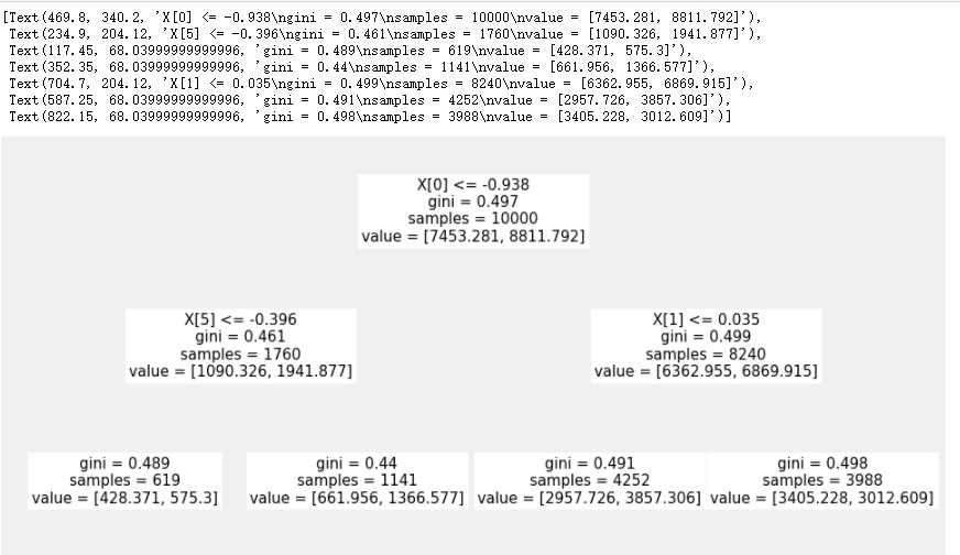

可以得到树的分裂图
同时也可以后续计算ITE，

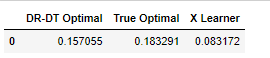
learner_x = BaseXRegressor(LGBMRegressor())
ite_x = learner_x.fit_predict(X=X, treatment=W, y=Y)pd.DataFrame({'DR-DT Optimal': [np.mean((policy_learner.predict(X) + 1) * tt / 2)],'True Optimal': [np.mean((np.sign(tt) + 1) * tt / 2)],'X Learner': [np.mean((np.sign(ite_x) + 1) * tt / 2)],
})

5 NN-Based的模型：dragonnet

基于神经网络的方法比较新，这里简单举一个例子——DragonNet。该方法主要工作是将propensity score估计和uplift score估计合并到一个网络实现。

首先，引述了可用倾向性得分代替X做ATE估计

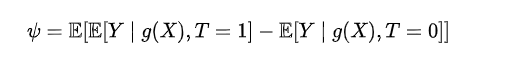
然后，为了准确预测ATE而非关注到Y预测上，我们应尽可能使用 X中与 T 相关的部分特征。
其中一种方法就是首先训练一个网络用X预测T，然后移除最后一层并接上Y的预测，则可以实现将X中与T相关的部分提取出来(即倾向性得分 $e$ 相关)，并用于Y的预测。
简单参考：【Uplift】建模方法篇

然后这里文档有两个数据集的应用，都在案例：dragonnet_example.ipynb，这里截取一个来简单看一下：

import pandas as pd
import numpy as np
from matplotlib import pyplot as plt
import seaborn as snsfrom sklearn.linear_model import LinearRegression
from sklearn.model_selection import train_test_split, StratifiedKFold
from sklearn.linear_model import LogisticRegressionCV, LogisticRegression
from xgboost import XGBRegressor
from lightgbm import LGBMRegressor
from sklearn.metrics import mean_absolute_error
from sklearn.metrics import mean_squared_error as mse
from scipy.stats import entropy
import warningsfrom causalml.inference.meta import LRSRegressor
from causalml.inference.meta import XGBTRegressor, MLPTRegressor
from causalml.inference.meta import BaseXRegressor, BaseRRegressor, BaseSRegressor, BaseTRegressor
from causalml.inference.tf import DragonNet
from causalml.match import NearestNeighborMatch, MatchOptimizer, create_table_one
from causalml.propensity import ElasticNetPropensityModel
from causalml.dataset.regression import *
from causalml.metrics import *import os, sys%matplotlib inlinewarnings.filterwarnings('ignore')
plt.style.use('fivethirtyeight')
sns.set_palette('Paired')
plt.rcParams['figure.figsize'] = (12,8)

数据载入，元数据在官方github上：

df = pd.read_csv(f'data/ihdp_npci_3.csv', header=None)
cols =  ["treatment", "y_factual", "y_cfactual", "mu0", "mu1"] + [f'x{i}' for i in range(1,26)]
df.columns = colsX = df.loc[:,'x1':]
treatment = df['treatment']
y = df['y_factual']
tau = df.apply(lambda d: d['y_factual'] - d['y_cfactual'] if d['treatment']==1 else d['y_cfactual'] - d['y_factual'], axis=1)

几个基础模型先跑一下然后对比：

p_model = ElasticNetPropensityModel()
p = p_model.fit_predict(X, treatment)s_learner = BaseSRegressor(LGBMRegressor())
s_ate = s_learner.estimate_ate(X, treatment, y)[0]
s_ite = s_learner.fit_predict(X, treatment, y)t_learner = BaseTRegressor(LGBMRegressor())
t_ate = t_learner.estimate_ate(X, treatment, y)[0][0]
t_ite = t_learner.fit_predict(X, treatment, y)x_learner = BaseXRegressor(LGBMRegressor())
x_ate = x_learner.estimate_ate(X, treatment, y, p)[0][0]
x_ite = x_learner.fit_predict(X, treatment, y, p)r_learner = BaseRRegressor(LGBMRegressor())
r_ate = r_learner.estimate_ate(X, treatment, y, p)[0][0]
r_ite = r_learner.fit_predict(X, treatment, y, p)

之后是DragonNet模型：

dragon = DragonNet(neurons_per_layer=200, targeted_reg=True)
dragon_ite = dragon.fit_predict(X, treatment, y, return_components=False)
dragon_ate = dragon_ite.mean()

训练的蛮快：

Train on 597 samples, validate on 150 samples
Epoch 1/30
597/597 [==============================] - 2s 3ms/sample - loss: 1239.5969 - regression_loss: 561.7198 - binary_classification_loss: 37.7623 - treatment_accuracy: 0.7590 - track_epsilon: 0.0339 - val_loss: 423.3901 - val_regression_loss: 156.0984 - val_binary_classification_loss: 33.2239 - val_treatment_accuracy: 0.7244 - val_track_epsilon: 0.0325
Epoch 2/30
597/597 [==============================] - 0s 71us/sample - loss: 290.8331 - regression_loss: 118.9768 - binary_classification_loss: 30.6743 - treatment_accuracy: 0.8561 - track_epsilon: 0.0319 - val_loss: 236.9888 - val_regression_loss: 84.3624 - val_binary_classification_loss: 34.7734 - val_treatment_accuracy: 0.7244 - val_track_epsilon: 0.0302
Epoch 3/30
597/597 [==============================] - 0s 69us/sample - loss: 232.0476 - regression_loss: 96.7705 - binary_classification_loss: 27.2036 - treatment_accuracy: 0.8529 - track_epsilon: 0.0301 - val_loss: 220.0190 - val_regression_loss: 71.6871 - val_binary_classification_loss: 37.6016 - val_treatment_accuracy: 0.7244 - val_track_epsilon: 0.0307
Epoch 4/30

最后几个模型一起来看一下：

df_preds = pd.DataFrame([s_ite.ravel(),t_ite.ravel(),x_ite.ravel(),r_ite.ravel(),dragon_ite.ravel(),tau.ravel(),treatment.ravel(),y.ravel()],index=['S','T','X','R','dragonnet','tau','w','y']).Tdf_cumgain = get_cumgain(df_preds)
df_result = pd.DataFrame([s_ate, t_ate, x_ate, r_ate, dragon_ate, tau.mean()],index=['S','T','X','R','dragonnet','actual'], columns=['ATE'])
df_result['MAE'] = [mean_absolute_error(t,p) for t,p in zip([s_ite, t_ite, x_ite, r_ite, dragon_ite],[tau.values.reshape(-1,1)]*5 )] + [None]
df_result['AUUC'] = auuc_score(df_preds)plot_gain(df_preds)

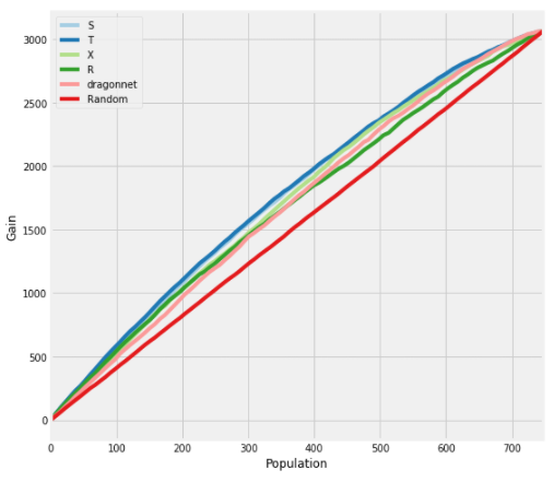
从AUUC来看，几个模型各有好坏

---

6 模型重要性 + SHAP

主要参考文档：feature_interpretations_example

里面内容比较多，就截取一些

import pandas as pd
import numpy as np
import matplotlib.pyplot as plt
from sklearn.ensemble import RandomForestRegressor, GradientBoostingRegressor
from sklearn.tree import DecisionTreeRegressor
from xgboost import XGBRegressor
from lightgbm import LGBMRegressorfrom causalml.inference.meta import BaseSRegressor, BaseTRegressor, BaseXRegressor, BaseRRegressor
from causalml.inference.tree import UpliftTreeClassifier, UpliftRandomForestClassifier
from causalml.dataset.regression import synthetic_data
from sklearn.linear_model import LinearRegressionimport shap
import matplotlib.pyplot as pltimport time
from sklearn.inspection import permutation_importance
from sklearn.model_selection import train_test_splitimport os
import warnings
warnings.filterwarnings('ignore')os.environ['KMP_DUPLICATE_LIB_OK'] = 'True'  # for lightgbm to work%reload_ext autoreload
%autoreload 2
%matplotlib inlineplt.style.use('fivethirtyeight')n_features = 25
n_samples = 10000
y, X, w, tau, b, e = synthetic_data(mode=1, n=n_samples, p=n_features, sigma=0.5)w_multi = np.array(['treatment_A' if x==1 else 'control' for x in w])
e_multi = {'treatment_A': e}feature_names = ['stars', 'tiger', 'merciful', 'quixotic', 'fireman', 'dependent','shelf', 'touch', 'barbarous', 'clammy', 'playground', 'rain', 'offer','cute', 'future', 'damp', 'nonchalant', 'change', 'rigid', 'sweltering','eight', 'wrap', 'lethal', 'adhesive', 'lip']  # specify feature namesmodel_tau = LGBMRegressor(importance_type='gain')  # specify model for model_tau

S-Learner为代表来看一下：

base_algo = LGBMRegressor()
# base_algo = XGBRegressor()
# base_algo = RandomForestRegressor()
# base_algo = LinearRegression()slearner = BaseSRegressor(base_algo, control_name='control')
slearner.estimate_ate(X, w_multi, y)slearner_tau = slearner.fit_predict(X, w_multi, y)
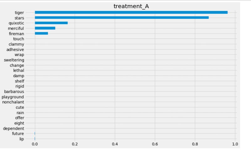
# 模型的重要性方法一：AUTO
slearner.plot_importance(X=X, tau=slearner_tau, normalize=True, method='auto', features=feature_names)# 重要性方法二：permutation方法
slearner.get_importance(X=X, tau=slearner_tau, method='permutation', features=feature_names, random_state=42)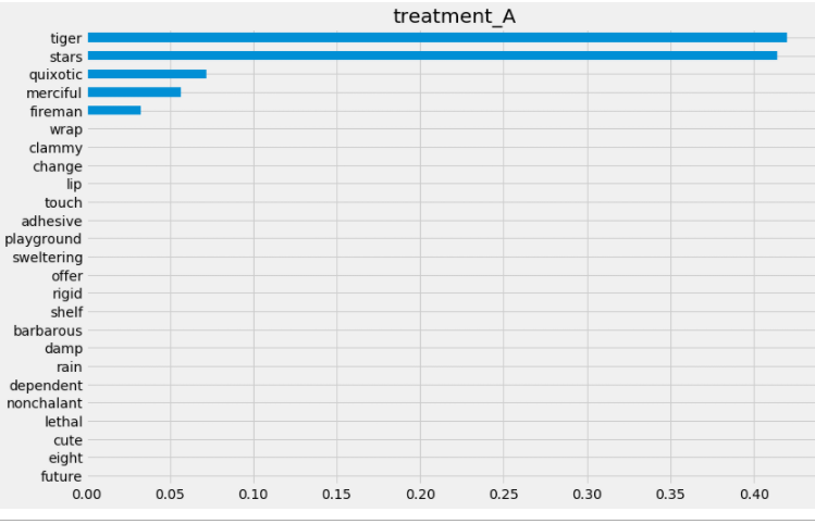

第二种：

SHAP值的计算：

shap_slearner = slearner.get_shap_values(X=X, tau=slearner_tau)
shap_slearner
# Plot shap values without specifying shap_dict
slearner.plot_shap_values(X=X, tau=slearner_tau, features=feature_names)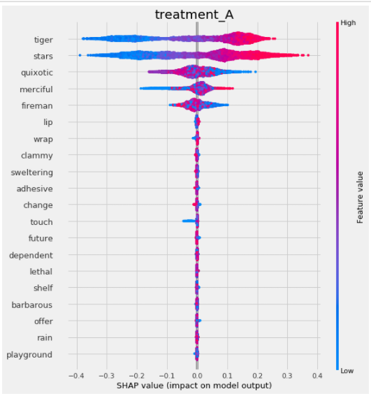

这篇关于因果推断笔记——因果图建模之Uber开源的CausalML（十二）的文章就介绍到这儿，希望我们推荐的文章对编程师们有所帮助！

---