RE2文本匹配调优实战

本文主要是介绍RE2文本匹配调优实战，希望对大家解决编程问题提供一定的参考价值，需要的开发者们随着小编来一起学习吧！

引言

在RE2文本匹配实战的最后，博主说过会结合词向量以及其他技巧来对效果进行调优，本篇文章对整个过程进行详细记录。其他文本匹配系列实战后续也会进行类似的调优，方法是一样的，不再赘述。

本文所用到的词向量可以在Gensim训练中文词向量实战文末找到，免费提供下载。

完整代码在文末。

数据准备

本次用的是LCQMC通用领域问题匹配数据集，它已经分好了训练、验证和测试集。

我们通过pandas来加载一下。

import pandas as pdtrain_df = pd.read_csv(data_path.format("train"), sep="\t", header=None, names=["sentence1", "sentence2", "label"])train_df.head()

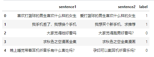
数据是长这样子的，有两个待匹配的句子，标签是它们是否相似。

下面用jieba来处理每个句子。

def tokenize(sentence):return list(jieba.cut(sentence))train_df.sentence1 = train_df.sentence1.apply(tokenize)
train_df.sentence2 = train_df.sentence2.apply(tokenize)

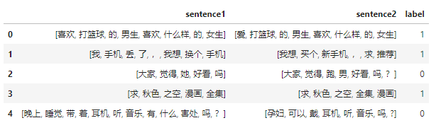
得到分好词的数据后，我们就可以得到整个训练语料库中的所有token：

train_sentences = train_df.sentence1.to_list() + train_df.sentence2.to_list()
train_sentences[0]

['喜欢', '打篮球', '的', '男生', '喜欢', '什么样', '的', '女生']

现在就可以来构建词表了，我们沿用之前的代码：

class Vocabulary:"""Class to process text and extract vocabulary for mapping"""def __init__(self, token_to_idx: dict = None, tokens: list[str] = None) -> None:"""Args:token_to_idx (dict, optional): a pre-existing map of tokens to indices. Defaults to None.tokens (list[str], optional): a list of unique tokens with no duplicates. Defaults to None."""assert any([tokens, token_to_idx]), "At least one of these parameters should be set as not None."if token_to_idx:self._token_to_idx = token_to_idxelse:self._token_to_idx = {}if PAD_TOKEN not in tokens:tokens = [PAD_TOKEN] + tokensfor idx, token in enumerate(tokens):self._token_to_idx[token] = idxself._idx_to_token = {idx: token for token, idx in self._token_to_idx.items()}self.unk_index = self._token_to_idx[UNK_TOKEN]self.pad_index = self._token_to_idx[PAD_TOKEN]@classmethoddef build(cls,sentences: list[list[str]],min_freq: int = 2,reserved_tokens: list[str] = None,) -> "Vocabulary":"""Construct the Vocabulary from sentencesArgs:sentences (list[list[str]]): a list of tokenized sequencesmin_freq (int, optional): the minimum word frequency to be saved. Defaults to 2.reserved_tokens (list[str], optional): the reserved tokens to add into the Vocabulary. Defaults to None.Returns:Vocabulary: a Vocubulary instane"""token_freqs = defaultdict(int)for sentence in tqdm(sentences):for token in sentence:token_freqs[token] += 1unique_tokens = (reserved_tokens if reserved_tokens else []) + [UNK_TOKEN]unique_tokens += [tokenfor token, freq in token_freqs.items()if freq >= min_freq and token != UNK_TOKEN]return cls(tokens=unique_tokens)def __len__(self) -> int:return len(self._idx_to_token)def __iter__(self):for idx, token in self._idx_to_token.items():yield idx, tokendef __getitem__(self, tokens: list[str] | str) -> list[int] | int:"""Retrieve the indices associated with the tokens or the index with the single tokenArgs:tokens (list[str] | str): a list of tokens or single tokenReturns:list[int] | int: the indices or the single index"""if not isinstance(tokens, (list, tuple)):return self._token_to_idx.get(tokens, self.unk_index)return [self.__getitem__(token) for token in tokens]def lookup_token(self, indices: list[int] | int) -> list[str] | str:"""Retrive the tokens associated with the indices or the token with the single indexArgs:indices (list[int] | int): a list of index or single indexReturns:list[str] | str: the corresponding tokens (or token)"""if not isinstance(indices, (list, tuple)):return self._idx_to_token[indices]return [self._idx_to_token[index] for index in indices]def to_serializable(self) -> dict:"""Returns a dictionary that can be serialized"""return {"token_to_idx": self._token_to_idx}@classmethoddef from_serializable(cls, contents: dict) -> "Vocabulary":"""Instantiates the Vocabulary from a serialized dictionaryArgs:contents (dict): a dictionary generated by `to_serializable`Returns:Vocabulary: the Vocabulary instance"""return cls(**contents)def __repr__(self):return f"<Vocabulary(size={len(self)})>"

主要修改是增加：

def __iter__(self):for idx, token in self._idx_to_token.items():yield idx, token

使得这个词表是可迭代的，其他代码参考完整代码。

模型实现

模型实现见RE2文本匹配实战，没有任何修改。

模型训练

主要优化在模型训练过程中，首先我们训练得更久——总epochs数设成50，同时我们引入早停策略，当模型不再优化则无需继续训练。

早停策略

class EarlyStopper:def __init__(self, patience: int = 5, mode: str = "min") -> None:self.patience = patienceself.counter = 0self.best_value = 0.0if mode not in {"min", "max"}:raise ValueError(f"mode {mode} is unknown!")self.mode = modedef step(self, value: float) -> bool:if self.is_better(value):self.best_value = valueself.counter = 0else:self.counter += 1if self.counter >= self.patience:return Truereturn Falsedef is_better(self, a: float) -> bool:if self.mode == "min":return a < self.best_valuereturn a > self.best_value

很简单，如果调用step()返回True，则触发了早停；通过best_value保存训练过程中的最佳指标，同时技术清零；其中patience表示最多忍耐模型不再优化次数；

学习率调度

当模型不再收敛时，还可以尝试减少学习率。这里引入的ReduceLROnPlateau就可以完成这件事。

lr_scheduler = ReduceLROnPlateau(optimizer, mode="max", factor=0.85, patience=0)for epoch in range(args.num_epochs):train(train_data_loader, model, criterion, optimizer, args.grad_clipping)acc, p, r, f1 = evaluate(dev_data_loader, model)# 当准确率不再下降，则降低学习率lr_scheduler.step(acc)

增加梯度裁剪值

梯度才才裁剪值增加到10.0。

载入预训练词向量

最重要的就是载入预训练词向量了：

def load_embedings(vocab, embedding_path: str, embedding_dim: int = 300, lower: bool = True
) -> list[list[float]]:word2vec = KeyedVectors.load_word2vec_format(embedding_path)embedding = np.random.randn(len(vocab), embedding_dim)load_count = 0for i, word in vocab:if lower:word = word.lower()if word in word2vec:embedding[i] = word2vec[word]load_count += 1print(f"loaded word count: {load_count}")return embedding.tolist()

首先加载word2vec文件；接着随机初始化一个词表大小的词向量；然后遍历(见上文)词表中的标记，如果标记出现在word2vec中，则使用word2vec的嵌入，并且计数加1；最后打印出工加载的标记数。

设定随机种子

def set_random_seed(seed: int = 666) -> None:np.random.seed(seed)torch.manual_seed(seed)torch.cuda.manual_seed_all(seed)

为了让结果可复现，还实现了设定随机种子，本文用的是 set_random_seed(seed=47)，最终能达到测试集上84.6%的准确率，实验过程中碰到了85.0%的准确率，但没有复现。

训练

训练参数：

Arguments : Namespace(dataset_csv='text_matching/data/lcqmc/{}.txt', vectorizer_file='vectorizer.json', model_state_file='model.pth', pandas_file='dataframe.{}.pkl', save_dir='/home/yjw/workspace/nlp-in-action-public/text_matching/re2/model_storage', reload_model=False, cuda=True, learning_rate=0.0005, batch_size=128, num_epochs=50, max_len=50, embedding_dim=300, hidden_size=150, encoder_layers=2, num_blocks=2, kernel_sizes=[3], dropout=0.2, min_freq=2, project_func='linear', grad_clipping=10.0, num_classes=2)

主要训练代码：

train_data_loader = DataLoader(train_dataset, batch_size=args.batch_size, shuffle=True
)
dev_data_loader = DataLoader(dev_dataset, batch_size=args.batch_size)
test_data_loader = DataLoader(test_dataset, batch_size=args.batch_size)optimizer = torch.optim.AdamW(model.parameters(), lr=args.learning_rate)
criterion = nn.CrossEntropyLoss()lr_scheduler = ReduceLROnPlateau(optimizer, mode="max", factor=0.85, patience=0)best_value = 0.0early_stopper = EarlyStopper(mode="max")for epoch in range(args.num_epochs):train(train_data_loader, model, criterion, optimizer, args.grad_clipping)acc, p, r, f1 = evaluate(dev_data_loader, model)lr_scheduler.step(acc)if acc > best_value:best_value = accprint(f"Save model with best acc :{acc:4f}")torch.save(model.state_dict(), model_save_path)if early_stopper.step(acc):print(f"Stop from early stopping.")breakacc, p, r, f1 = evaluate(dev_data_loader, model)print(f"EVALUATE [{epoch+1}/{args.num_epochs}]  accuracy={acc:.3f} precision={p:.3f} recal={r:.3f} f1 score={f1:.4f}")model.eval()acc, p, r, f1 = evaluate(test_data_loader, model)
print(f"TEST accuracy={acc:.3f} precision={p:.3f} recal={r:.3f} f1 score={f1:.4f}")model.load_state_dict(torch.load(model_save_path))
model.to(device)
acc, p, r, f1 = evaluate(test_data_loader, model)
print(f"TEST[best score] accuracy={acc:.3f} precision={p:.3f} recal={r:.3f} f1 score={f1:.4f}"
)

输出：

Arguments : Namespace(dataset_csv='text_matching/data/lcqmc/{}.txt', vectorizer_file='vectorizer.json', model_state_file='model.pth', pandas_file='dataframe.{}.pkl', save_dir='/home/yjw/workspace/nlp-in-action-public/text_matching/re2/model_storage', reload_model=False, cuda=True, learning_rate=0.0005, batch_size=128, num_epochs=50, max_len=50, embedding_dim=300, hidden_size=150, encoder_layers=2, num_blocks=2, kernel_sizes=[3], dropout=0.2, min_freq=2, project_func='linear', grad_clipping=10.0, num_classes=2)
Using device: cuda:0.
Loads cached dataframes.
Loads vectorizer file.
set_count: 4789
Model: RE2((embedding): Embedding((embedding): Embedding(4827, 300, padding_idx=0)(dropout): Dropout(p=0.2, inplace=False))(connection): AugmentedResidualConnection()(blocks): ModuleList((0): ModuleDict((encoder): Encoder((encoders): ModuleList((0): Conv1d((model): ModuleList((0): Sequential((0): Conv1d(300, 150, kernel_size=(3,), stride=(1,), padding=(1,))(1): GeLU())))(1): Conv1d((model): ModuleList((0): Sequential((0): Conv1d(150, 150, kernel_size=(3,), stride=(1,), padding=(1,))(1): GeLU()))))(dropout): Dropout(p=0.2, inplace=False))(alignment): Alignment((projection): Sequential((0): Dropout(p=0.2, inplace=False)(1): Linear((model): Sequential((0): Linear(in_features=450, out_features=150, bias=True)(1): GeLU()))))(fusion): Fusion((dropout): Dropout(p=0.2, inplace=False)(fusion1): Linear((model): Sequential((0): Linear(in_features=900, out_features=150, bias=True)(1): GeLU()))(fusion2): Linear((model): Sequential((0): Linear(in_features=900, out_features=150, bias=True)(1): GeLU()))(fusion3): Linear((model): Sequential((0): Linear(in_features=900, out_features=150, bias=True)(1): GeLU()))(fusion): Linear((model): Sequential((0): Linear(in_features=450, out_features=150, bias=True)(1): GeLU()))))(1): ModuleDict((encoder): Encoder((encoders): ModuleList((0): Conv1d((model): ModuleList((0): Sequential((0): Conv1d(450, 150, kernel_size=(3,), stride=(1,), padding=(1,))(1): GeLU())))(1): Conv1d((model): ModuleList((0): Sequential((0): Conv1d(150, 150, kernel_size=(3,), stride=(1,), padding=(1,))(1): GeLU()))))(dropout): Dropout(p=0.2, inplace=False))(alignment): Alignment((projection): Sequential((0): Dropout(p=0.2, inplace=False)(1): Linear((model): Sequential((0): Linear(in_features=600, out_features=150, bias=True)(1): GeLU()))))(fusion): Fusion((dropout): Dropout(p=0.2, inplace=False)(fusion1): Linear((model): Sequential((0): Linear(in_features=1200, out_features=150, bias=True)(1): GeLU()))(fusion2): Linear((model): Sequential((0): Linear(in_features=1200, out_features=150, bias=True)(1): GeLU()))(fusion3): Linear((model): Sequential((0): Linear(in_features=1200, out_features=150, bias=True)(1): GeLU()))(fusion): Linear((model): Sequential((0): Linear(in_features=450, out_features=150, bias=True)(1): GeLU())))))(pooling): Pooling()(prediction): Prediction((dense): Sequential((0): Dropout(p=0.2, inplace=False)(1): Linear((model): Sequential((0): Linear(in_features=600, out_features=150, bias=True)(1): GeLU()))(2): Dropout(p=0.2, inplace=False)(3): Linear((model): Sequential((0): Linear(in_features=150, out_features=2, bias=True)(1): GeLU()))))
)
New modelTRAIN iter=1866 loss=0.436723: 100%|██████████| 1866/1866 [01:55<00:00, 16.17it/s]
100%|██████████| 69/69 [00:01<00:00, 40.39it/s]
Save model with best accuracy :0.771302
EVALUATE [2/50]  accuracy=0.771 precision=0.800 recal=0.723 f1 score=0.7598TRAIN iter=1866 loss=0.403501: 100%|██████████| 1866/1866 [01:57<00:00, 15.93it/s]
100%|██████████| 69/69 [00:01<00:00, 45.32it/s]
Save model with best accuracy :0.779709
EVALUATE [3/50]  accuracy=0.780 precision=0.785 recal=0.770 f1 score=0.7777TRAIN iter=1866 loss=0.392297: 100%|██████████| 1866/1866 [01:45<00:00, 17.64it/s]
100%|██████████| 69/69 [00:01<00:00, 43.32it/s]
Save model with best accuracy :0.810838
EVALUATE [4/50]  accuracy=0.811 precision=0.804 recal=0.822 f1 score=0.8130TRAIN iter=1866 loss=0.383858: 100%|██████████| 1866/1866 [01:46<00:00, 17.52it/s]
100%|██████████| 69/69 [00:01<00:00, 42.72it/s]
EVALUATE [5/50]  accuracy=0.810 precision=0.807 recal=0.816 f1 score=0.8113TRAIN iter=1866 loss=0.374672: 100%|██████████| 1866/1866 [01:46<00:00, 17.55it/s]
100%|██████████| 69/69 [00:01<00:00, 44.62it/s]
Save model with best accuracy :0.816746
EVALUATE [6/50]  accuracy=0.817 precision=0.818 recal=0.815 f1 score=0.8164TRAIN iter=1866 loss=0.369444: 100%|██████████| 1866/1866 [01:46<00:00, 17.52it/s]
100%|██████████| 69/69 [00:01<00:00, 45.27it/s]
EVALUATE [7/50]  accuracy=0.815 precision=0.800 recal=0.842 f1 score=0.8203TRAIN iter=1866 loss=0.361552: 100%|██████████| 1866/1866 [01:47<00:00, 17.39it/s]
100%|██████████| 69/69 [00:01<00:00, 42.68it/s]
Save model with best accuracy :0.824926
EVALUATE [8/50]  accuracy=0.825 precision=0.820 recal=0.832 f1 score=0.8262TRAIN iter=1866 loss=0.358231: 100%|██████████| 1866/1866 [01:50<00:00, 16.95it/s]
100%|██████████| 69/69 [00:01<00:00, 42.80it/s]
Save model with best accuracy :0.827312
EVALUATE [9/50]  accuracy=0.827 precision=0.841 recal=0.808 f1 score=0.8239TRAIN iter=1866 loss=0.354693: 100%|██████████| 1866/1866 [01:55<00:00, 16.19it/s]
100%|██████████| 69/69 [00:01<00:00, 36.67it/s]
Save model with best accuracy :0.830607
EVALUATE [10/50]  accuracy=0.831 precision=0.818 recal=0.851 f1 score=0.8340TRAIN iter=1866 loss=0.351138: 100%|██████████| 1866/1866 [02:02<00:00, 15.23it/s]
100%|██████████| 69/69 [00:02<00:00, 32.18it/s]
Save model with best accuracy :0.837991
EVALUATE [11/50]  accuracy=0.838 precision=0.840 recal=0.836 f1 score=0.8376TRAIN iter=1866 loss=0.348067: 100%|██████████| 1866/1866 [01:52<00:00, 16.57it/s]
100%|██████████| 69/69 [00:01<00:00, 42.16it/s]
EVALUATE [12/50]  accuracy=0.836 precision=0.836 recal=0.837 f1 score=0.8365TRAIN iter=1866 loss=0.343886: 100%|██████████| 1866/1866 [02:09<00:00, 14.43it/s]
100%|██████████| 69/69 [00:02<00:00, 32.44it/s]
Save model with best accuracy :0.839127
EVALUATE [13/50]  accuracy=0.839 precision=0.838 recal=0.841 f1 score=0.8395TRAIN iter=1866 loss=0.341275: 100%|██████████| 1866/1866 [02:17<00:00, 13.60it/s]
100%|██████████| 69/69 [00:02<00:00, 32.74it/s]
Save model with best accuracy :0.842649
EVALUATE [14/50]  accuracy=0.843 precision=0.841 recal=0.845 f1 score=0.8431TRAIN iter=1866 loss=0.339279: 100%|██████████| 1866/1866 [02:15<00:00, 13.74it/s]
100%|██████████| 69/69 [00:01<00:00, 42.64it/s]
Save model with best accuracy :0.846399
EVALUATE [15/50]  accuracy=0.846 precision=0.858 recal=0.831 f1 score=0.8440TRAIN iter=1866 loss=0.338046: 100%|██████████| 1866/1866 [01:49<00:00, 17.00it/s]
100%|██████████| 69/69 [00:01<00:00, 42.64it/s]
EVALUATE [16/50]  accuracy=0.844 precision=0.844 recal=0.843 f1 score=0.8436TRAIN iter=1866 loss=0.334223: 100%|██████████| 1866/1866 [01:59<00:00, 15.60it/s]
100%|██████████| 69/69 [00:02<00:00, 32.00it/s]
EVALUATE [17/50]  accuracy=0.844 precision=0.836 recal=0.855 f1 score=0.8455TRAIN iter=1866 loss=0.331690: 100%|██████████| 1866/1866 [02:04<00:00, 15.01it/s]
100%|██████████| 69/69 [00:01<00:00, 42.16it/s]
EVALUATE [18/50]  accuracy=0.844 precision=0.834 recal=0.860 f1 score=0.8465TRAIN iter=1866 loss=0.328178: 100%|██████████| 1866/1866 [01:49<00:00, 16.98it/s]
100%|██████████| 69/69 [00:01<00:00, 42.50it/s]
EVALUATE [19/50]  accuracy=0.845 precision=0.842 recal=0.849 f1 score=0.8454TRAIN iter=1866 loss=0.326720: 100%|██████████| 1866/1866 [01:48<00:00, 17.12it/s]
100%|██████████| 69/69 [00:01<00:00, 41.95it/s]
Save model with best accuracy :0.847421
EVALUATE [20/50]  accuracy=0.847 precision=0.844 recal=0.853 f1 score=0.8482TRAIN iter=1866 loss=0.324938: 100%|██████████| 1866/1866 [01:49<00:00, 16.99it/s]
100%|██████████| 69/69 [00:01<00:00, 43.29it/s]
EVALUATE [21/50]  accuracy=0.845 precision=0.842 recal=0.848 f1 score=0.8452TRAIN iter=1866 loss=0.322923: 100%|██████████| 1866/1866 [01:48<00:00, 17.24it/s]
100%|██████████| 69/69 [00:01<00:00, 43.47it/s]
EVALUATE [22/50]  accuracy=0.847 precision=0.844 recal=0.852 f1 score=0.8480TRAIN iter=1866 loss=0.322150: 100%|██████████| 1866/1866 [01:46<00:00, 17.51it/s]
100%|██████████| 69/69 [00:01<00:00, 42.77it/s]
Save model with best accuracy :0.849920
EVALUATE [23/50]  accuracy=0.850 precision=0.839 recal=0.866 f1 score=0.8523TRAIN iter=1866 loss=0.320312: 100%|██████████| 1866/1866 [01:49<00:00, 17.06it/s]
100%|██████████| 69/69 [00:01<00:00, 41.91it/s]
EVALUATE [24/50]  accuracy=0.847 precision=0.843 recal=0.853 f1 score=0.8479TRAIN iter=1866 loss=0.319144: 100%|██████████| 1866/1866 [01:49<00:00, 17.00it/s]
100%|██████████| 69/69 [00:01<00:00, 42.76it/s]
EVALUATE [25/50]  accuracy=0.849 precision=0.841 recal=0.861 f1 score=0.8511TRAIN iter=1866 loss=0.318375: 100%|██████████| 1866/1866 [01:48<00:00, 17.20it/s]
100%|██████████| 69/69 [00:01<00:00, 43.52it/s]
EVALUATE [26/50]  accuracy=0.850 precision=0.843 recal=0.859 f1 score=0.8512TRAIN iter=1866 loss=0.317125: 100%|██████████| 1866/1866 [01:48<00:00, 17.17it/s]
100%|██████████| 69/69 [00:01<00:00, 42.54it/s]
EVALUATE [27/50]  accuracy=0.848 precision=0.841 recal=0.857 f1 score=0.8490TRAIN iter=1866 loss=0.316708: 100%|██████████| 1866/1866 [01:49<00:00, 17.03it/s]
100%|██████████| 69/69 [00:01<00:00, 42.04it/s]
Stop from early stopping.
100%|██████████| 98/98 [00:02<00:00, 38.74it/s]
TEST accuracy=0.846 precision=0.792 recal=0.938 f1 score=0.8587
100%|██████████| 98/98 [00:02<00:00, 39.47it/s]
TEST[best f1] accuracy=0.846 precision=0.793 recal=0.939 f1 score=0.8594

一些结论