本文主要是介绍机器学习之线性分类以及Fisher线性判别,希望对大家解决编程问题提供一定的参考价值,需要的开发者们随着小编来一起学习吧!
机器学习之线性分类以及Fisher线性判别
一、什么是线性分类器和Fisher判别
在机器学习领域,分类的目标是指将具有相似特征的对象聚集。而一个线性分类器则透过特征的线性组合来做出分类决定,以达到此种目的。对象的特征通常被描述为特征值,而在向量中则描述为特征向量。
线性分类器定义:

Fisher线性判别:
Fisher判别法是判别分析的方法之一,它是借助于方差分析的思想,利用已知各总体抽取的样品的p维观察值构造一个或多个线性判别函数y=l′x其中l= (l1,l2…lp)′,x= (x1,x2,…,xp)′,使不同总体之间的离差(记为B)尽可能地大,而同一总体内的离差(记为E)尽可能地小来确定判别系数l=(l1,l2…lp)′。数学上证明判别系数l恰好是|B-λE|=0的特征根,记为λ1≥λ2≥…≥λr>0。所对应的特征向量记为l1,l2,…lr,则可写出多个相应的线性判别函数,在有些问题中,仅用一个λ1对应的特征向量l1所构成线性判别函数y1=l′1x不能很好区分各个总体时,可取λ2对应的特征向量l′2建立第二个线性判别函数y2=l′2x,如还不够,依此类推。有了判别函数,再人为规定一个分类原则(有加权法和不加权法等)就可对新样品x判别所属 。
基本介绍:

两个总体的Fisher判别函数:


多个总体的Fisher判别函数:

判别规则:
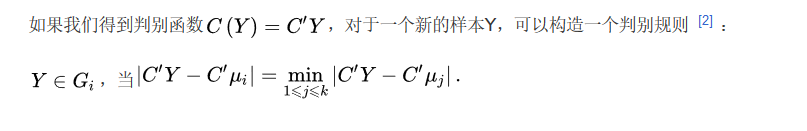
二、判别下一模式属于哪类


三、Fisher判别python代码的推导
Iris数据集的 Fisher线性分类判断及准确率计算:
#导入相关库
import pandas as pd
import numpy as np
import matplotlib.pyplot as plt
import seaborn as sns
#构建数据集
path=(r'http://archive.ics.uci.edu/ml/machine-learning-databases/iris/iris.data')
df = pd.read_csv(path, header=0)
Iris1=df.values[0:50,0:4]
Iris2=df.values[50:100,0:4]
Iris3=df.values[100:150,0:4]
#构建样本类内离散度矩阵
m1=np.mean(Iris1,axis=0)
m2=np.mean(Iris2,axis=0)
m3=np.mean(Iris3,axis=0)
s1=np.zeros((4,4))
s2=np.zeros((4,4))
s3=np.zeros((4,4))
for i in range(0,30,1):a=Iris1[i,:]-m1a=np.array([a])b=a.Ts1=s1+np.dot(b,a)
for i in range(0,30,1):c=Iris2[i,:]-m2c=np.array([c])d=c.Ts2=s2+np.dot(d,c)
for i in range(0,30,1):a=Iris3[i,:]-m3a=np.array([a])b=a.Ts3=s3+np.dot(b,a)
sw12=s1+s2
sw13=s1+s3
sw23=s2+s3
#投影方向
a=np.array([m1-m2])
sw12=np.array(sw12,dtype='float')
sw13=np.array(sw13,dtype='float')
sw23=np.array(sw23,dtype='float')
#判别函数以及T
a=m1-m2
a=np.array([a])
a=a.T
b=m1-m3
b=np.array([b])
b=b.T
c=m2-m3
c=np.array([c])
c=c.T
w12=(np.dot(np.linalg.inv(sw12),a)).T
w13=(np.dot(np.linalg.inv(sw13),b)).T
w23=(np.dot(np.linalg.inv(sw23),c)).T
T12=-0.5*(np.dot(np.dot((m1+m2),np.linalg.inv(sw12)),a))
T13=-0.5*(np.dot(np.dot((m1+m3),np.linalg.inv(sw13)),b))
T23=-0.5*(np.dot(np.dot((m2+m3),np.linalg.inv(sw23)),c))
#通过判别函数进行判别,求解正确率
kind1=0
kind2=0
kind3=0
newiris1=[]
newiris2=[]
newiris3=[]
for i in range(30,49):x=Iris1[i,:]x=np.array([x])g12=np.dot(w12,x.T)+T12g13=np.dot(w13,x.T)+T13g23=np.dot(w23,x.T)+T23if g12>0 and g13>0:newiris1.extend(x)kind1=kind1+1elif g12<0 and g23>0:newiris2.extend(x)elif g13<0 and g23<0 :newiris3.extend(x)
for i in range(30,49):x=Iris2[i,:]x=np.array([x])g12=np.dot(w12,x.T)+T12g13=np.dot(w13,x.T)+T13g23=np.dot(w23,x.T)+T23if g12>0 and g13>0:newiris1.extend(x)elif g12<0 and g23>0:newiris2.extend(x)kind2=kind2+1elif g13<0 and g23<0 :newiris3.extend(x)
for i in range(30,49):x=Iris3[i,:]x=np.array([x])g12=np.dot(w12,x.T)+T12g13=np.dot(w13,x.T)+T13g23=np.dot(w23,x.T)+T23if g12>0 and g13>0:newiris1.extend(x)elif g12<0 and g23>0:     newiris2.extend(x)elif g13<0 and g23<0 :newiris3.extend(x)kind3=kind3+1
correct=(kind1+kind2+kind3)/60
print("样本类内离散度矩阵S1:",s1,'\n')
print("样本类内离散度矩阵S2:",s2,'\n')
print("样本类内离散度矩阵S3:",s3,'\n')
print("总体类内离散度矩阵Sw12:",sw12,'\n')
print("总体类内离散度矩阵Sw13:",sw13,'\n')
print("总体类内离散度矩阵Sw23:",sw23,'\n')
print('判断出来的综合正确率:',correct*100,'%')
样本类内离散度矩阵S1: [[4.084080000000003 2.9814400000000005 0.54099999999999950.4941599999999999][2.9814400000000005 3.6879200000000028 -0.0250000000000004280.5628800000000002][0.5409999999999995 -0.025000000000000428 1.0829999999999995 0.19][0.4941599999999999 0.5628800000000002 0.19 0.30832000000000004]] 样本类内离散度矩阵S2: [[8.316120000000005 2.7365199999999987 5.5689600000000031.7302799999999998][2.7365199999999987 3.09192 2.49916 1.3588799999999999][5.568960000000003 2.49916 6.258680000000002 2.2232399999999997][1.7302799999999998 1.3588799999999999 2.22323999999999971.3543200000000004]] 样本类内离散度矩阵S3: [[14.328471470220745 3.1402832153269435 11.946005830903791.3147563515201988][3.1402832153269435 3.198721366097457 2.2396501457725931.2317617659308615][11.94600583090379 2.239650145772593 11.6008163265306181.4958892128279884][1.3147563515201988 1.2317617659308615 1.49588921282798841.6810578925447726]] 总体类内离散度矩阵Sw12: [[12.4002 5.71796 6.10996 2.22444][ 5.71796 6.77984 2.47416 1.92176][ 6.10996 2.47416 7.34168 2.41324][ 2.22444 1.92176 2.41324 1.66264]] 总体类内离散度矩阵Sw13: [[18.41255147 6.12172322 12.48700583 1.80891635][ 6.12172322 6.88664137 2.21465015 1.79464177][12.48700583 2.21465015 12.68381633 1.68588921][ 1.80891635 1.79464177 1.68588921 1.98937789]] 总体类内离散度矩阵Sw23: [[22.64459147 5.87680322 17.51496583 3.04503635][ 5.87680322 6.29064137 4.73881015 2.59064177][17.51496583 4.73881015 17.85949633 3.71912921][ 3.04503635 2.59064177 3.71912921 3.03537789]] 判断出来的综合正确率: 91.66666666666666 %
四、Iris数据集的线性分类以及数据可视化
Iris数据集的线性分类以及数据可视化
#导入相关库
import numpy as np
from sklearn.linear_model import LogisticRegression
import matplotlib.pyplot as plt
import matplotlib as mpl
from sklearn import preprocessing
import pandas as pd
from sklearn.preprocessing import StandardScaler
from sklearn.pipeline import Pipeline
#读取数据
df = pd.read_csv('http://archive.ics.uci.edu/ml/machine-learning-databases/iris/iris.data', header=0)
x = df.values[:, :-1]
y = df.values[:, -1]
le = preprocessing.LabelEncoder()
le.fit(['Iris-setosa', 'Iris-versicolor', 'Iris-virginica'])
y = le.transform(y)
#构建线性模型
x = x[:, :2]
x = StandardScaler().fit_transform(x)
lr = LogisticRegression()   # Logistic回归模型
lr.fit(x, y.ravel())        # 根据数据[x,y],计算回归参数
C:\Users\Administrator\Anaconda3\lib\site-packages\sklearn\linear_model\logistic.py:432: FutureWarning: Default solver will be changed to 'lbfgs' in 0.22. Specify a solver to silence this warning.FutureWarning)
C:\Users\Administrator\Anaconda3\lib\site-packages\sklearn\linear_model\logistic.py:469: FutureWarning: Default multi_class will be changed to 'auto' in 0.22. Specify the multi_class option to silence this warning."this warning.", FutureWarning)LogisticRegression(C=1.0, class_weight=None, dual=False, fit_intercept=True,intercept_scaling=1, l1_ratio=None, max_iter=100,multi_class='warn', n_jobs=None, penalty='l2',random_state=None, solver='warn', tol=0.0001, verbose=0,warm_start=False)
#分类及可视化
N, M = 500, 500     # 横纵各采样多少个值
x1_min, x1_max = x[:, 0].min(), x[:, 0].max()   # 第0列的范围
x2_min, x2_max = x[:, 1].min(), x[:, 1].max()   # 第1列的范围
t1 = np.linspace(x1_min, x1_max, N)
t2 = np.linspace(x2_min, x2_max, M)
x1, x2 = np.meshgrid(t1, t2)                    # 生成网格采样点
x_test = np.stack((x1.flat, x2.flat), axis=1)   # 测试点
cm_light = mpl.colors.ListedColormap(['#77E0A0', '#FF8080', '#A0A0FF'])
cm_dark = mpl.colors.ListedColormap(['g', 'r', 'b'])
y_hat = lr.predict(x_test)       # 预测值
y_hat = y_hat.reshape(x1.shape)                 # 使之与输入的形状相同
plt.pcolormesh(x1, x2, y_hat, cmap=cm_light)     # 预测值的显示
plt.scatter(x[:, 0], x[:, 1], c=y.ravel(), edgecolors='k', s=50, cmap=cm_dark)
plt.xlabel('petal length')
plt.ylabel('petal width')
plt.xlim(x1_min, x1_max)
plt.ylim(x2_min, x2_max)
plt.grid()
plt.savefig('iris.png')
plt.show()
#计算准确率
y_hat = lr.predict(x)
y = y.reshape(-1)
result = y_hat == y
acc = np.mean(result)
print('准确度: %.2f%%' % (100 * acc))

准确度: 79.19%
可以看到,鸢尾花数据集共分为三类,并且不同的数据分布在不同的类别之中,从而达到线性分类器的效果,但是准确率并不高只有79.19%。
数据可视化
from sklearn import datasets
import pandas as pd
import matplotlib.pyplot as plt
import numpy as np
import seaborn as sns
from mpl_toolkits.mplot3d import Axes3D
iris = datasets.load_iris()
data1=pd.DataFrame(np.concatenate((iris.data,iris.target.reshape(150,1)),axis=1),columns=np.append(iris.feature_names,'target'))
data1
| sepal length (cm) | sepal width (cm) | petal length (cm) | petal width (cm) | target | |
|---|---|---|---|---|---|
| 0 | 5.1 | 3.5 | 1.4 | 0.2 | 0.0 |
| 1 | 4.9 | 3.0 | 1.4 | 0.2 | 0.0 |
| 2 | 4.7 | 3.2 | 1.3 | 0.2 | 0.0 |
| 3 | 4.6 | 3.1 | 1.5 | 0.2 | 0.0 |
| 4 | 5.0 | 3.6 | 1.4 | 0.2 | 0.0 |
| ... | ... | ... | ... | ... | ... |
| 145 | 6.7 | 3.0 | 5.2 | 2.3 | 2.0 |
| 146 | 6.3 | 2.5 | 5.0 | 1.9 | 2.0 |
| 147 | 6.5 | 3.0 | 5.2 | 2.0 | 2.0 |
| 148 | 6.2 | 3.4 | 5.4 | 2.3 | 2.0 |
| 149 | 5.9 | 3.0 | 5.1 | 1.8 | 2.0 |
150 rows × 5 columns
data=pd.DataFrame(np.concatenate((iris.data,np.repeat(iris.target_names,50).reshape(150,1)),axis=1),columns=np.append(iris.feature_names,'target'))
data=data.apply(pd.to_numeric,errors='ignore')
data
| sepal length (cm) | sepal width (cm) | petal length (cm) | petal width (cm) | target | |
|---|---|---|---|---|---|
| 0 | 5.1 | 3.5 | 1.4 | 0.2 | setosa |
| 1 | 4.9 | 3.0 | 1.4 | 0.2 | setosa |
| 2 | 4.7 | 3.2 | 1.3 | 0.2 | setosa |
| 3 | 4.6 | 3.1 | 1.5 | 0.2 | setosa |
| 4 | 5.0 | 3.6 | 1.4 | 0.2 | setosa |
| ... | ... | ... | ... | ... | ... |
| 145 | 6.7 | 3.0 | 5.2 | 2.3 | virginica |
| 146 | 6.3 | 2.5 | 5.0 | 1.9 | virginica |
| 147 | 6.5 | 3.0 | 5.2 | 2.0 | virginica |
| 148 | 6.2 | 3.4 | 5.4 | 2.3 | virginica |
| 149 | 5.9 | 3.0 | 5.1 | 1.8 | virginica |
150 rows × 5 columns
sns.pairplot(data.iloc[:,[0,1,4]],hue='target')
sns.pairplot(data.iloc[:,2:5],hue='target')
<seaborn.axisgrid.PairGrid at 0x200fa6d6388>


plt.scatter(data1.iloc[:,0],data1.iloc[:,1],c=data1.target)
plt.xlabel('sepal length (cm)')
plt.ylabel('sepal width (cm)')
Text(0, 0.5, 'sepal width (cm)')

这篇关于机器学习之线性分类以及Fisher线性判别的文章就介绍到这儿,希望我们推荐的文章对编程师们有所帮助!


