机器学习实战：基于sklearn的工业蒸汽量预测

本文主要是介绍机器学习实战：基于sklearn的工业蒸汽量预测，希望对大家解决编程问题提供一定的参考价值，需要的开发者们随着小编来一起学习吧！

写在前面

本期内容：基于机器学习的工业蒸汽量预测

实验环境：
anaconda
python
sklearn

注：本专栏内所有文章都包含完整代码以及数据集

工业蒸汽量预测

1.基础代码

（1）导入工具包

import numpy as np
import pandas as pd
import matplotlib.pyplot as plt
import seaborn as sns
from scipy import stats
import warnings
warnings.filterwarnings("ignore")
from sklearn.linear_model import LinearRegression  # 多元线性回归
from sklearn.linear_model import SGDRegressor      # SGD回归
from sklearn.neighbors import KNeighborsRegressor  # KNN最近邻
from sklearn.tree import DecisionTreeRegressor     # 决策树
from sklearn.ensemble import RandomForestRegressor # 随机森林
from sklearn.svm import SVR                        # 支持向量机
import lightgbm as lgb                             
from sklearn.model_selection import train_test_split
from sklearn.metrics import mean_squared_error
from sklearn import preprocessing
from sklearn.preprocessing import PolynomialFeatures

这些库是Python中的数据分析、机器学习和统计学习等方面常用的库。

• numpy：提供了对于矩阵、数组等数值运算的支持。
• pandas：提供了高效的数据结构，允许快速处理和操作数据。
• matplotlib：Python中最著名的绘图库，用于绘制各种类型的图形。
• seaborn：基于matplotlib的数据可视化库，可帮助用户更好地理解数据并探索数据集。
• scipy：提供了科学计算领域所需的各种算法，例如数值积分、插值、优化和线性代数等。
• warnings：提供了忽略警告的相关函数。
• scikit-learn：提供了各种常用的机器学习算法和数据预处理方法。
• lightgbm：轻量级机器学习库，支持梯度 boosting 决策树等算法。
• preprocessing：提供了各种数据预处理工具，例如标准化、缩放、归一化和编码等。
• PolynomialFeatures：用于将原有特征转化为多项式特征，从而使得模型能够更好地拟合数据。

（2）读取数据

train_data_file = "zhengqi_data/zhengqi_train.txt"
test_data_file = "zhengqi_data/zhengqi_test.txt"
train_data = pd.read_csv(train_data_file, sep='\t', encoding='utf-8')
test_data = pd.read_csv(test_data_file, sep='\t', encoding='utf-8')

这段代码读取了两个数据文件：zhengqi_train.txt和zhengqi_test.txt，并将数据分别保存到了train_data和test_data两个变量中。

其中，sep='\t'指定了数据文件使用制表符作为分隔符进行分隔，encoding='utf-8'指定了数据文件使用UTF-8编码。

这段代码中使用了pandas库中的read_csv函数对数据进行读取，并将其解析为DataFrame格式。

这段代码的目的是读取训练数据和测试数据，为接下来的数据分析和建模做准备。

（3）归一化处理

features_columns = [col for col in train_data.columns if col not in ['target']]
min_max_scaler = preprocessing.MinMaxScaler()
train_data_scaler = min_max_scaler.fit_transform(train_data[features_columns])
test_data_scaler = min_max_scaler.fit_transform(test_data[features_columns])
train_data_scaler = pd.DataFrame(train_data_scaler)
train_data_scaler.columns = features_columns
test_data_scaler = pd.DataFrame(test_data_scaler)
test_data_scaler.columns = features_columns
train_data_scaler['target'] = train_data['target']

这段代码中首先定义了features_columns变量，其值是训练数据中除去target列的所有列名，也就是所有特征的列名。

接着，使用preprocessing模块中的MinMaxScaler()函数创建了一个最小最大值标准化的数据缩放器，用来将数据按照最小最大值进行标准化处理。

然后，对训练数据和测试数据中的特征数据进行缩放处理，并分别保存到train_data_scaler和test_data_scaler两个变量中。缩放处理后的数据都被转换成了DataFrame格式，并且列名也被指定为features_columns中的特征列名。

最后，为了方便后续建模处理，又将缩放处理后的训练数据和原始训练数据中的target列合并到了一个DataFrame中，即train_data_scaler中的最后一列是原始训练数据中的target列。这样方便我们在建模时直接使用整个数据集进行训练。

（4）PCA处理

from sklearn.decomposition import PCA
pca = PCA(n_components=16)
new_train_pca_16 = pca.fit_transform(train_data_scaler.iloc[:, 0:-1])
new_test_pca_16 = pca.transform(test_data_scaler)
new_train_pca_16 = pd.DataFrame(new_train_pca_16)
new_test_pca_16 = pd.DataFrame(new_test_pca_16)
new_train_pca_16['target'] = train_data_scaler['target']

这段代码首先导入了PCA模块，并创建了一个PCA对象，设置n_components参数为16，表示希望降维后的特征数为16。

然后对训练数据和测试数据进行降维处理，其中训练数据通过fit_transform()函数进行降维，测试数据只能通过transform()函数进行降维，这是由于fit_transform()是基于训练数据集进行的，而测试数据集中可能会出现新的特征，因此只能使用已经训练好的PCA对象对测试数据进行降维。

接着，将降维后的训练数据和测试数据都转换成DataFrame格式，并向降维后的训练数据中添加target列，方便后续的建模。最后得到的new_train_pca_16就是降维后的训练数据集，new_test_pca_16则是降维后的测试数据集。

（5）切分数据

new_train_pca_16 = new_train_pca_16.fillna(0)
train = new_train_pca_16[new_test_pca_16.columns]
target = new_train_pca_16['target']
train_data, test_data, train_target, test_target = train_test_split(train, target, test_size=0.2, random_state=0)

这段代码首先对降维后的训练数据集new_train_pca_16进行缺失值填充，将所有缺失值填充为0。

然后，根据测试数据集new_test_pca_16的特征列，从降维后的训练数据集new_train_pca_16中提取相应的特征列和目标列，生成训练数据集train和目标值target。

接着，使用train_test_split()函数将训练数据集train和目标值target按照指定比例（这里为0.2）进行划分，得到了新的训练集train_data、测试集test_data，以及它们的目标值train_target和test_target。这一步是为了进行模型的训练和调试，可以使用训练集进行模型的训练，再使用测试集进行模型的评估。

2.模型训练

（1）多元线性回归

clf = LinearRegression()
clf.fit(train_data, train_target)
test_pred = clf.predict(test_data)
loss = mean_squared_error(test_target, test_pred)
score = clf.score(test_data, test_target)
print("LinearRegression loss：", loss)
print("LinearRegression score：", score)

LinearRegression loss： 0.1419036258610617
LinearRegression score： 0.8634398527356705

这段代码定义了一个线性回归模型clf，并使用训练集train_data和目标值train_target对其进行拟合训练。接着，使用predict()函数对测试集test_data进行预测，并计算预测结果与真实目标值test_target之间的均方误差（Mean Squared Error，MSE），即mean_squared_error()，并将结果赋值给loss。

最后，计算模型在测试集上的得分（score），即$R^2$决定系数（coefficient of determination），表示模型对测试集数据的拟合程度，值越接近1，则说明模型预测效果越好。使用score()函数计算$R^2$，并将结果赋值给score，最后打印输出loss和score的值。

综合起来，这段代码是对线性回归模型进行训练和评估，通过均方误差和得分来评价模型的预测效果。

（2）支持向量机

clf = SVR()
clf.fit(train_data, train_target)
test_pred = clf.predict(test_data)
loss = mean_squared_error(test_target, test_pred)
score = clf.score(test_data, test_target)
print("SVR loss：", loss)
print("SVR score：", score)

SVR loss： 0.1467083314287438
SVR score： 0.8588160716595842

这段代码使用了支持向量机回归模型（Support Vector Regression，SVR）来进行模型训练和预测。其中，首先定义了一个SVR模型clf，接着使用训练集train_data和目标值train_target对其进行拟合训练。然后，使用predict()函数对测试集test_data进行预测，并计算预测结果与真实目标值test_target之间的均方误差（Mean Squared Error，MSE），即mean_squared_error()，并将结果赋值给loss。

最后，计算模型在测试集上的得分（score），即$R^2$决定系数（coefficient of determination），表示模型对测试集数据的拟合程度，值越接近1，则说明模型预测效果越好。使用score()函数计算$R^2$，并将结果赋值给score，最后打印输出loss和score的值。

综合起来，这段代码是对SVR模型进行训练和评估，通过均方误差和得分来评价模型的预测效果。

（3）决策树

from sklearn.tree import DecisionTreeRegressor
clf = DecisionTreeRegressor()
clf.fit(train_data, train_target)
test_pred = clf.predict(test_data)
loss = mean_squared_error(test_target, test_pred)
score = clf.score(test_data, test_target)
print("DecisionTreeRegressor loss：", loss)
print("DecisionTreeRegressor score：", score)

DecisionTreeRegressor loss： 0.3219484238754325
DecisionTreeRegressor score： 0.6901747653791848

这段代码使用了决策树回归模型（Decision Tree Regression）来进行模型训练和预测。其中，首先定义了一个决策树回归模型clf，接着使用训练集train_data和目标值train_target对其进行拟合训练。然后，使用predict()函数对测试集test_data进行预测，并计算预测结果与真实目标值test_target之间的均方误差（Mean Squared Error，MSE），即mean_squared_error()，并将结果赋值给loss。

最后，计算模型在测试集上的得分（score），即$R^2$决定系数（coefficient of determination），表示模型对测试集数据的拟合程度，值越接近1，则说明模型预测效果越好。使用score()函数计算$R^2$，并将结果赋值给score，最后打印输出loss和score的值。

综合起来，这段代码是对决策树回归模型进行训练和评估，通过均方误差和得分来评价模型的预测效果。

（4）随机森林回归

clf = RandomForestRegressor(n_estimators=200)
clf.fit(train_data, train_target)
test_pred = clf.predict(test_data)
loss = mean_squared_error(test_target, test_pred)
score = clf.score(test_data, test_target)
print("RandomForestRegressor loss：", loss)
print("RandomForestRegressor score：", score)

RandomForestRegressor loss： 0.1533863238125865
RandomForestRegressor score： 0.8523895436703662

这段代码使用了随机森林回归模型（Random Forest Regression）来进行模型训练和预测。其中，首先定义了一个随机森林回归模型clf，并设置了森林中决策树的数量n_estimators=200。接着使用训练集train_data和目标值train_target对其进行拟合训练。然后，使用predict()函数对测试集test_data进行预测，并计算预测结果与真实目标值test_target之间的均方误差（Mean Squared Error，MSE），即mean_squared_error()，并将结果赋值给loss。

最后，计算模型在测试集上的得分（score），即$R^2$决定系数（coefficient of determination），表示模型对测试集数据的拟合程度，值越接近1，则说明模型预测效果越好。使用score()函数计算$R^2$，并将结果赋值给score，最后打印输出loss和score的值。

综合起来，这段代码是对随机森林回归模型进行训练和评估，通过均方误差和得分来评价模型的预测效果。由于随机森林模型同时考虑多个决策树的结果，能够有效降低预测方差，从而提高模型的预测效果。

（5）LGB模型回归

warnings.filterwarnings('ignore')
clf = lgb.LGBMRegressor(learning_rate=0.01,max_depth=3,n_estimators=5000,boosting_type='gbdt',random_state=2023,objective='regression',
)
clf.fit(X=train_data, y=train_target, eval_metric='MSE')
test_pred = clf.predict(test_data)
loss = mean_squared_error(test_target, test_pred)
score = clf.score(test_data, test_target)
print("LightGBM loss：", loss)
print("LightGBM score：", score)

LightGBM loss： 0.14156298447523044
LightGBM score： 0.8637676670359125

这段代码使用了 LightGBM 回归模型（Light Gradient Boosting Machine Regression）。该模型是一种梯度提升决策树（Gradient Boosting Decision Tree）算法，在训练过程中采用了直方图算法来加快训练速度，同时使用了按叶子结点统计的直方图做决策，减少了计算量。

在具体实现上，该代码首先使用LGBMRegressor()函数定义了一个 LightGBM 回归模型clf，设置了模型的一些超参数，包括学习率（learning_rate）、最大深度（max_depth）、迭代次数（n_estimators）、提升类型（boosting_type）、随机种子（random_state）和目标函数（objective）。接着，使用训练集train_data和目标值train_target对其进行拟合训练，并设置了评估指标为均方误差。然后，使用predict()函数对测试集test_data进行预测，并计算预测结果与真实目标值test_target之间的均方误差（Mean Squared Error，MSE），即mean_squared_error()，并将结果赋值给loss。

最后，计算模型在测试集上的得分（score），即$R^2$决定系数（coefficient of determination），表示模型对测试集数据的拟合程度，值越接近1，则说明模型预测效果越好。使用score()函数计算$R^2$，并将结果赋值给score，最后打印输出loss和score的值。

综合起来，这段代码是对 LightGBM 回归模型进行训练和评估，通过均方误差和得分来评价模型的预测效果。由于 LightGBM 算法运行速度快、效果好，可以在大规模数据集上高效地优化模型，因此在实际工程场景中比较常用。

3.模型正则化

（1）L2范数正则化

poly = PolynomialFeatures(3)
train_data_poly = poly.fit_transform(train_data)
test_data_poly = poly.transform(test_data)
clf = SGDRegressor(max_iter=1000, tol=1e-3, penalty='l2', alpha=0.0001)
clf.fit(train_data_poly, train_target)
train_pred = clf.predict(train_data_poly)
test_pred = clf.predict(test_data_poly)
loss_train = mean_squared_error(train_target, train_pred)
loss_test = mean_squared_error(test_target, test_pred)
score_train = clf.score(train_data_poly, train_target)
score_test = clf.score(test_data_poly, test_target)
print("SGDRegressor train MSE：", loss_train)
print("SGDRegressor test MSE：", loss_test)
print("SGDRegressor train score：", score_train)
print("SGDRegressor test score：", score_test)

SGDRegressor train MSE： 0.1339159145514598
SGDRegressor test MSE： 0.14238772543844233
SGDRegressor train score： 0.8590386590525457
SGDRegressor test score： 0.8629739822607158

np.savetxt('L2正则化.txt', clf.predict(poly.transform(new_test_pca_16)).reshape(-1,1))

这段代码使用了 SGDRegressor 回归模型（Stochastic Gradient Descent Regression）。该模型是一种随机梯度下降法（Stochastic Gradient Descent）的线性回归算法，其训练过程中使用了 mini-batch 实现批量操作，同时采用了正则化技巧以避免过拟合。

在具体实现上，该代码首先使用PolynomialFeatures()函数将原始数据进行多项式特征转换，将每个特征的幂次从1开始一直转换到指定的最高次数，这里设置为3，得到一个新的数据集train_data_poly和test_data_poly。接着，使用SGDRegressor()函数定义了一个 SGD 回归模型clf，设置了模型的一些超参数，包括迭代次数（max_iter）、收敛阈值（tol）、正则化方式（penalty）和正则化强度（alpha）。然后，使用fit()函数对多项式特征转换后的训练集train_data_poly和目标值train_target进行拟合训练。

接下来，使用predict()函数对训练集train_data_poly和测试集test_data_poly进行预测，并计算预测结果与真实目标值train_target和test_target之间的均方误差（Mean Squared Error，MSE），并将结果分别赋值给loss_train和loss_test。接着，计算训练集和测试集上的得分（score），即$R^2$决定系数，表示模型对训练集和测试集数据的拟合程度，值越接近1，则说明模型预测效果越好。使用score()函数计算$R^2$，并将结果分别赋值给score_train和score_test。最后打印输出训练集和测试集的均方误差和得分。

综合起来，这段代码是对 SGDRegressor 回归模型进行训练和评估，通过多项式特征转换和正则化技巧提高模型的预测能力，通过均方误差和得分来评价模型的预测效果。由于 SGDRegressor 模型具有训练速度快、内存占用小等优点，在处理大规模数据集时较为高效。

（2）L1范数正则化

poly = PolynomialFeatures(3)
train_data_poly = poly.fit_transform(train_data)
test_data_poly = poly.transform(test_data)
clf = SGDRegressor(max_iter=1000, tol=1e-3, penalty='l1', alpha=0.0001)
clf.fit(train_data_poly, train_target)
train_pred = clf.predict(train_data_poly)
test_pred = clf.predict(test_data_poly)
loss_train = mean_squared_error(train_target, train_pred)
loss_test = mean_squared_error(test_target, test_pred)
score_train = clf.score(train_data_poly, train_target)
score_test = clf.score(test_data_poly, test_target)
print("SGDRegressor train MSE：", loss_train)
print("SGDRegressor test MSE：", loss_test)
print("SGDRegressor train score：", score_train)
print("SGDRegressor test score：", score_test)

SGDRegressor train MSE： 0.1349906641770775
SGDRegressor test MSE： 0.14315596332614164
SGDRegressor train score： 0.8579073659652582
SGDRegressor test score： 0.8622346728988748

这段代码与上一段代码相比，唯一的区别在于正则化方式不同，这里采用了 L1 正则化（L1 regularization）。

L1 正则化是一种常用的正则化技巧，可以有效地用于特征选择和降维等问题。它通过在损失函数中增加对参数向量绝对值的惩罚项，促使大部分参数变为0，从而删除一些无关特征，以及为后续建模提供更加简洁的特征集。

具体实现上，代码与上一段代码基本一致。不同之处在于，在定义 SGD 回归模型时，penalty的取值为l1，表示采用 L1 正则化；同时，与 L2 正则化相比，L1 正则化会更倾向于将某些参数压缩到0的位置，因此会更适合稀疏性较高的数据集。

最后输出训练集和测试集的均方误差和得分。

（3）ElasticNet联合L1和L2范数加权正则化

poly = PolynomialFeatures(3)
train_data_poly = poly.fit_transform(train_data)
test_data_poly = poly.transform(test_data)
clf = SGDRegressor(max_iter=1000, tol=1e-3, penalty='elasticnet', alpha=0.0001)
clf.fit(train_data_poly, train_target)
train_pred = clf.predict(train_data_poly)
test_pred = clf.predict(test_data_poly)
loss_train = mean_squared_error(train_target, train_pred)
loss_test = mean_squared_error(test_target, test_pred)
score_train = clf.score(train_data_poly, train_target)
score_test = clf.score(test_data_poly, test_target)
print("SGDRegressor train MSE：", loss_train)
print("SGDRegressor test MSE：", loss_test)
print("SGDRegressor train score：", score_train)
print("SGDRegressor test score：", score_test)

SGDRegressor train MSE： 0.1341138913851733
SGDRegressor test MSE： 0.14237841112120603
SGDRegressor train score： 0.8588302664947959
SGDRegressor test score： 0.8629829458409325

这段代码与之前两段代码相比，唯一的区别在于正则化方式采用了弹性网络正则化（elastic net regularization）。

弹性网络正则化是将 L1 正则化和 L2 正则化相结合的一种正则化方法。它能够同时产生稀疏性和平滑性，既能够处理稀疏问题，又能够适当地保留一些相关特征。

具体实现上，代码与之前两段代码基本一致。不同之处在于，在定义 SGD 回归模型时，penalty的取值为elasticnet，表示采用弹性网络正则化；同时，我们需要调节L1_ratio这个参数，来控制 L1 正则化和 L2 正则化的权重比例。在这里我们默认L1_ratio为0.5，表示 L1 正则化和 L2 正则化的权重比例相同。

最后输出训练集和测试集的均方误差和得分。

4.模型交叉验证

（1）简单交叉验证

from sklearn.model_selection import train_test_split
train_data, test_data, train_target, test_target = train_test_split(train, target, test_size=0.2, random_state=0)
clf = SGDRegressor(max_iter=1000, tol=1e-3)
clf.fit(train_data, train_target)
train_pred = clf.predict(train_data)
test_pred = clf.predict(test_data)
loss_train = mean_squared_error(train_target, train_pred)
loss_test = mean_squared_error(test_target, test_pred)
score_train = clf.score(train_data, train_target)
score_test = clf.score(test_data, test_target)
print("SGDRegressor train MSE：", loss_train)
print("SGDRegressor test MSE：", loss_test)
print("SGDRegressor train score：", score_train)
print("SGDRegressor test score：", score_test)

SGDRegressor train MSE： 0.14148181620679126
SGDRegressor test MSE： 0.14686800506596273
SGDRegressor train score： 0.8510747090889865
SGDRegressor test score： 0.8586624106429573

这段代码中，我们使用了train_test_split()函数将数据集划分为训练集和测试集。其中，train和target分别表示原始数据集和目标标签，test_size=0.2表示将数据集按8:2的比例划分为训练集和测试集，random_state=0表示随机状态。

接着，我们定义了一个SGDRegressor模型，将其拟合训练集数据，并进行预测。最后计算训练集和测试集的均方误差和得分，并输出结果。

（2）K折交叉验证

from sklearn.model_selection import KFold
kf = KFold(n_splits=5)
for k, (train_index, test_index) in enumerate(kf.split(train)):train_data, test_data, train_target, test_target = train.values[train_index], train.values[test_index], target[train_index], target[test_index]clf = SGDRegressor(max_iter=1000, tol=1e-3)clf.fit(train_data, train_target)train_pred = clf.predict(train_data)test_pred = clf.predict(test_data)loss_train = mean_squared_error(train_target, train_pred)loss_test = mean_squared_error(test_target, test_pred)score_train = clf.score(train_data, train_target)score_test = clf.score(test_data, test_target)print("第", k, "折：")print("SGDRegressor train MSE：", loss_train)print("SGDRegressor test MSE：", loss_test)print("SGDRegressor train score：", score_train)print("SGDRegressor test score：", score_test)

第 0 折：
SGDRegressor train MSE： 0.14999880405646862
SGDRegressor test MSE： 0.10592525937102415
SGDRegressor train score： 0.8465710522678433
SGDRegressor test score： 0.8785882684927748
第 1 折：
SGDRegressor train MSE： 0.13362245515687662
SGDRegressor test MSE： 0.18229509115449283
SGDRegressor train score： 0.8551005648227722
SGDRegressor test score： 0.8352528732421299
第 2 折：
SGDRegressor train MSE： 0.1471021092885928
SGDRegressor test MSE： 0.13280652017602562
SGDRegressor train score： 0.8496732158633719
SGDRegressor test score： 0.8556298799895657
第 3 折：
SGDRegressor train MSE： 0.14087834722612338
SGDRegressor test MSE： 0.16353154781238963
SGDRegressor train score： 0.8547916380218887
SGDRegressor test score： 0.8142748394425501
第 4 折：
SGDRegressor train MSE： 0.13804889017571664
SGDRegressor test MSE： 0.16512488568551079
SGDRegressor train score： 0.8592892787632107
SGDRegressor test score： 0.8176784985924272

这段代码中，我们使用了KFold函数进行交叉验证，将数据集划分为5个互不重叠的训练集和测试集组合。其中，n_splits=5表示划分为5个组合，train_index和test_index分别表示当前组合的训练集和测试集索引。

然后，我们在循环中定义了一个SGDRegressor模型，并用当前组合的训练集数据进行拟合和预测。接着，计算训练集和测试集的均方误差和得分，并输出结果。

需要注意的是，由于数据集被划分为5个组合，因此KFold函数会对同一模型进行5次训练和测试，最终输出每次训练和测试的结果。这样可以更客观地评估模型的性能，并减少因为随机划分数据集而引入的偏差。

（3）留一法交叉验证

from sklearn.model_selection import LeaveOneOut
loo = LeaveOneOut()
num = 100
for k, (train_index, test_index) in enumerate(loo.split(train)):train_data, test_data, train_target, test_target = train.values[train_index], train.values[test_index], target[train_index], target[test_index]clf = SGDRegressor(max_iter=1000, tol=1e-3)clf.fit(train_data, train_target)train_pred = clf.predict(train_data)test_pred = clf.predict(test_data)loss_train = mean_squared_error(train_target, train_pred)loss_test = mean_squared_error(test_target, test_pred)score_train = clf.score(train_data, train_target)score_test = clf.score(test_data, test_target)print("第", k, "个：")print("SGDRegressor train MSE：", loss_train)print("SGDRegressor test MSE：", loss_test)print("SGDRegressor train score：", score_train)print("SGDRegressor test score：", score_test)if k > 9:break

第 0 个：
SGDRegressor train MSE： 0.14159231038900896
SGDRegressor test MSE： 0.01277094911992315
SGDRegressor train score： 0.8537553053677902
SGDRegressor test score： nan
第 1 个：
SGDRegressor train MSE： 0.1409611114988628
SGDRegressor test MSE： 0.11808753778871625
SGDRegressor train score： 0.8543916238696744
SGDRegressor test score： nan
第 2 个：
SGDRegressor train MSE： 0.1416105880760475
SGDRegressor test MSE： 0.037395746566420834
SGDRegressor train score： 0.8537231131215837
SGDRegressor test score： nan
第 3 个：
SGDRegressor train MSE： 0.1416319810809687
SGDRegressor test MSE： 0.003879737915583517
SGDRegressor train score： 0.8537141229751738
SGDRegressor test score： nan
第 4 个：
SGDRegressor train MSE： 0.1415566889516793
SGDRegressor test MSE： 0.012622642331936025
SGDRegressor train score： 0.8537887475079426
SGDRegressor test score： nan
第 5 个：
SGDRegressor train MSE： 0.1415347464062493
SGDRegressor test MSE： 0.1391720073804877
SGDRegressor train score： 0.8538146542385079
SGDRegressor test score： nan
第 6 个：
SGDRegressor train MSE： 0.14168663870602863
SGDRegressor test MSE： 0.02514154676355979
SGDRegressor train score： 0.853653637839331
SGDRegressor test score： nan
第 7 个：
SGDRegressor train MSE： 0.14159938732202335
SGDRegressor test MSE： 0.0007110487070548562
SGDRegressor train score： 0.8537359259211437
SGDRegressor test score： nan
第 8 个：
SGDRegressor train MSE： 0.1415121451335673
SGDRegressor test MSE： 0.08899215853332627
SGDRegressor train score： 0.8538000107354135
SGDRegressor test score： nan
第 9 个：
SGDRegressor train MSE： 0.14160761847464748
SGDRegressor test MSE： 0.049347443459542464
SGDRegressor train score： 0.8537145735785513
SGDRegressor test score： nan
第 10 个：
SGDRegressor train MSE： 0.14158927093686474
SGDRegressor test MSE： 0.006824179048538113
SGDRegressor train score： 0.8537290718497261
SGDRegressor test score： nan

这段代码中，使用了LeaveOneOut函数进行留一法交叉验证。留一法交叉验证是将数据集中的每个数据点都作为测试集进行测试，而其余数据点作为训练集进行训练，因此需要进行非常多次的训练和测试。在这段代码中，我们仅对前100个数据进行留一法交叉验证。

循环中的代码与KFold中的代码类似，区别在于每次只留一个数据点作为测试集，并将剩余数据点作为训练集进行拟合和预测。最后输出每个测试集的均方误差和得分。

需要注意的是，由于留一法交叉验证需要进行非常多次训练和测试，因此运行时间会比较长。此外，如果使用的数据集比较大，留一法也会造成计算资源的浪费。因此，一般情况下，我们更多地使用’KFold’函数进行交叉验证。

（4）留P法交叉验证

from sklearn.model_selection import LeavePOut
lpo = LeavePOut(p=10)
num = 100
for k, (train_index, test_index) in enumerate(lpo.split(train)):train_data, test_data, train_target, test_target = train.values[train_index], train.values[test_index], target[train_index], target[test_index]clf = SGDRegressor(max_iter=1000, tol=1e-3)clf.fit(train_data, train_target)train_pred = clf.predict(train_data)test_pred = clf.predict(test_data)loss_train = mean_squared_error(train_target, train_pred)loss_test = mean_squared_error(test_target, test_pred)score_train = clf.score(train_data, train_target)score_test = clf.score(test_data, test_target)print("第", k, "个：")print("SGDRegressor train MSE：", loss_train)print("SGDRegressor test MSE：", loss_test)print("SGDRegressor train score：", score_train)print("SGDRegressor test score：", score_test)if k > 9:break

第 0 个：
SGDRegressor train MSE： 0.1413793567015725
SGDRegressor test MSE： 0.04873755890347202
SGDRegressor train score： 0.8543175999817231
SGDRegressor test score： 0.3901616039644231
第 1 个：
SGDRegressor train MSE： 0.1418672871013134
SGDRegressor test MSE： 0.04457078953481626
SGDRegressor train score： 0.8538103568428461
SGDRegressor test score： 0.46961787061218296
第 2 个：
SGDRegressor train MSE： 0.1418697509979678
SGDRegressor test MSE： 0.04564378700057346
SGDRegressor train score： 0.8537899771306875
SGDRegressor test score： 0.5553508462189696
第 3 个：
SGDRegressor train MSE： 0.1418678680288433
SGDRegressor test MSE： 0.054210648559559926
SGDRegressor train score： 0.8537608414800607
SGDRegressor test score： 0.8111712794305601
第 4 个：
SGDRegressor train MSE： 0.14188403460372054
SGDRegressor test MSE： 0.0693633867417041
SGDRegressor train score： 0.8536563953162203
SGDRegressor test score： 0.8528271565838054
第 5 个：
SGDRegressor train MSE： 0.14204867363316417
SGDRegressor test MSE： 0.04519490065418205
SGDRegressor train score： 0.8536243340435593
SGDRegressor test score： 0.737790260906185
第 6 个：
SGDRegressor train MSE： 0.14197603878786572
SGDRegressor test MSE： 0.04950900176151719
SGDRegressor train score： 0.8536113076105263
SGDRegressor test score： 0.865619940173157
第 7 个：
SGDRegressor train MSE： 0.14196108627919937
SGDRegressor test MSE： 0.054049265494149526
SGDRegressor train score： 0.8537317137595262
SGDRegressor test score： 0.5733504224863128
第 8 个：
SGDRegressor train MSE： 0.14188795095216164
SGDRegressor test MSE： 0.04741584943138243
SGDRegressor train score： 0.8536580997439611
SGDRegressor test score： 0.8968290870324733
第 9 个：
SGDRegressor train MSE： 0.14205466083946663
SGDRegressor test MSE： 0.04504203563745397
SGDRegressor train score： 0.8536080933235433
SGDRegressor test score： 0.7712153359789988
第 10 个：
SGDRegressor train MSE： 0.14188392087224969
SGDRegressor test MSE： 0.05398520720528875
SGDRegressor train score： 0.8538187452287642
SGDRegressor test score： 0.4716854719367686

这段代码中，使用了LeavePOut函数进行交叉验证。与LeaveOneOut不同的是，LeavePOut每次留下p个数据作为测试集进行交叉验证。在这段代码中，我们将p设为10，因此每次留下10个数据点进行验证。同样地，我们仅对前100个数据进行验证。

循环中的代码与LeaveOneOut和KFold中的代码类似，区别在于每次留下10个数据点作为测试集，并将剩余的数据点作为训练集进行拟合和预测。最后输出每个测试集的均方误差和得分。

需要注意的是，LeavePOut需要指定参数p，这个参数的取值需要根据数据集的大小和计算资源的限制来确定。如果p过大，会导致计算开销过大，如果p过小，则可能导致预测结果不够准确。通常情况下，我们会根据经验和实验调整p的取值。

5.模型超参空间及调参

（1）穷举网格搜索

from sklearn.model_selection import GridSearchCV, train_test_split
from sklearn.ensemble import RandomForestRegressor
train_data, test_data, train_target, test_target = train_test_split(train, target, test_size=0.2, random_state=0)
randomForestRegressor = RandomForestRegressor()
parameters = {'n_estimators':[50, 100, 200], 'max_depth':[1, 2, 3]}
clf = GridSearchCV(randomForestRegressor, parameters, cv=5)
clf.fit(train_data, train_target)
loss_test = mean_squared_error(test_target, clf.predict(test_data))
print("RandomForestRegressor GridSearchCV test MSE：", loss_test)
sorted(clf.cv_results_.keys())

RandomForestRegressor GridSearchCV test MSE： 0.2568225281378069
['mean_fit_time','mean_score_time','mean_test_score','param_max_depth','param_n_estimators','params','rank_test_score','split0_test_score','split1_test_score','split2_test_score','split3_test_score','split4_test_score','std_fit_time','std_score_time','std_test_score']

这段代码中，我们使用了GridSearchCV函数进行模型选择和参数调优，具体步骤如下：

1. 首先使用train_test_split函数将数据集划分为训练集和测试集。

2. 创建一个RandomForestRegressor对象作为基础模型。

3. 定义参数空间parameters，包括两个参数n_estimators和max_depth，分别表示树的数量和树的深度。我们指定了3个树的数量和3个树的深度，因此总共有9种参数组合。

4. 创建一个GridSearchCV对象，将基础模型和参数空间作为参数传入，同时指定交叉验证的折数为5（即5折交叉验证）。

5. 调用GridSearchCV对象的fit方法，进行模型选择和参数调优。在这个过程中，GridSearchCV对象会在参数空间中搜索不同的参数组合，并对每个组合进行交叉验证，最终选择出平均得分最高的最优模型和参数组合。

6. 使用测试集对最优模型进行评估，并输出均方误差。

7. 最后一行代码输出了cv_results_.keys()，即交叉验证结果的各个属性值（例如训练时间、测试时间、得分等），并按字母顺序排序。这些属性值可以用于分析交叉验证的结果，例如得分的均值和标准差等。

需要注意的是，GridSearchCV需要进行的计算量较大，特别是当参数空间较大时，可能需要较长的计算时间。因此，在实际应用中，我们需要根据实际情况和计算资源的限制来确定参数空间和交叉验证的折数，以保证计算效率和结果准确性的平衡。

（2）随机参数优化

from sklearn.model_selection import RandomizedSearchCV, train_test_split
from sklearn.ensemble import RandomForestRegressor
train_data, test_data, train_target, test_target = train_test_split(train, target, test_size=0.2, random_state=0)
randomForestRegressor = RandomForestRegressor()
parameters = {'n_estimators':[50, 100, 200, 300],'max_depth':[1, 2, 3, 4, 5]
}
clf = RandomizedSearchCV(randomForestRegressor, parameters, cv=5)
clf.fit(train_data, train_target)
loss_test = mean_squared_error(test_target, clf.predict(test_data))
print("RandomForestRegressor RandomizedSearchCV test MSE：", loss_test)
sorted(clf.cv_results_.keys())

RandomForestRegressor RandomizedSearchCV test MSE： 0.1964024324240653
['mean_fit_time','mean_score_time','mean_test_score','param_max_depth','param_n_estimators','params','rank_test_score','split0_test_score','split1_test_score','split2_test_score','split3_test_score','split4_test_score','std_fit_time','std_score_time','std_test_score']

这段代码中，我们使用了RandomizedSearchCV函数进行模型选择和参数调优，与GridSearchCV不同的是，RandomizedSearchCV将在指定的参数空间中进行随机搜索，而不是穷举搜索所有可能的参数组合。具体步骤如下：

1. 首先使用train_test_split函数将数据集划分为训练集和测试集。

2. 创建一个RandomForestRegressor对象作为基础模型。

3. 定义参数空间parameters，包括两个参数n_estimators和max_depth，分别表示树的数量和树的深度。我们指定了4个树的数量和5个树的深度，因此总共有20种参数组合。

4. 创建一个RandomizedSearchCV对象，将基础模型和参数空间作为参数传入，同时指定交叉验证的折数为5（即5折交叉验证）。

5. 调用RandomizedSearchCV对象的fit方法，进行模型选择和参数调优。在这个过程中，RandomizedSearchCV对象会在指定的参数空间中随机搜索一定次数的参数组合，并对每个组合进行交叉验证，最终选择出平均得分最高的最优模型和参数组合。

6. 使用测试集对最优模型进行评估，并输出均方误差。

7. 最后一行代码输出了cv_results_.keys()，即交叉验证结果的各个属性值（例如训练时间、测试时间、得分等），并按字母顺序排序。这些属性值可以用于分析交叉验证的结果，例如得分的均值和标准差等。

需要注意的是，与GridSearchCV类似，RandomizedSearchCV需要进行的计算量较大，特别是当参数空间较大时，可能需要较长的计算时间。因此，在实际应用中，我们需要根据实际情况和计算资源的限制来确定参数空间、搜索次数和交叉验证的折数，以保证计算效率和结果准确性的平衡。

（3）LGB调参

clf = lgb.LGBMRegressor(num_leaves=31)
parameters = {'learning_rate': [0.01, 0.1, 1], 'n_estimators': [20, 40]}
clf = GridSearchCV(clf, parameters, cv=5)
clf.fit(train_data, train_target)
print('Best parameters found by grid search are：', clf.best_params_)
loss_test = mean_squared_error(test_target, clf.predict(test_data))
print("LGBMRegressor GridSearchCV test MSE：", loss_test)

[LightGBM] [Warning] Auto-choosing col-wise multi-threading, the overhead of testing was 0.000238 seconds.
You can set `force_col_wise=true` to remove the overhead.
[LightGBM] [Info] Total Bins 4080
[LightGBM] [Info] Number of data points in the train set: 1848, number of used features: 16
[LightGBM] [Info] Start training from score 0.113883
[LightGBM] [Warning] Auto-choosing col-wise multi-threading, the overhead of testing was 0.000167 seconds.
You can set `force_col_wise=true` to remove the overhead.
[LightGBM] [Info] Total Bins 4080
[LightGBM] [Info] Number of data points in the train set: 1848, number of used features: 16
[LightGBM] [Info] Start training from score 0.124781
[LightGBM] [Warning] Auto-choosing col-wise multi-threading, the overhead of testing was 0.000172 seconds.
You can set `force_col_wise=true` to remove the overhead.
[LightGBM] [Info] Total Bins 4080
[LightGBM] [Info] Number of data points in the train set: 1848, number of used features: 16
[LightGBM] [Info] Start training from score 0.129659
[LightGBM] [Warning] Auto-choosing col-wise multi-threading, the overhead of testing was 0.000166 seconds.
You can set `force_col_wise=true` to remove the overhead.
[LightGBM] [Info] Total Bins 4080
[LightGBM] [Info] Number of data points in the train set: 1848, number of used features: 16
[LightGBM] [Info] Start training from score 0.128611
[LightGBM] [Warning] Auto-choosing col-wise multi-threading, the overhead of testing was 0.000165 seconds.
You can set `force_col_wise=true` to remove the overhead.
[LightGBM] [Info] Total Bins 4080
[LightGBM] [Info] Number of data points in the train set: 1848, number of used features: 16
[LightGBM] [Info] Start training from score 0.134065
[LightGBM] [Warning] Auto-choosing col-wise multi-threading, the overhead of testing was 0.000204 seconds.
You can set `force_col_wise=true` to remove the overhead.
[LightGBM] [Info] Total Bins 4080
[LightGBM] [Info] Number of data points in the train set: 1848, number of used features: 16
[LightGBM] [Info] Start training from score 0.113883
[LightGBM] [Warning] Auto-choosing col-wise multi-threading, the overhead of testing was 0.000189 seconds.
You can set `force_col_wise=true` to remove the overhead.
[LightGBM] [Info] Total Bins 4080
[LightGBM] [Info] Number of data points in the train set: 1848, number of used features: 16
[LightGBM] [Info] Start training from score 0.124781
[LightGBM] [Warning] Auto-choosing col-wise multi-threading, the overhead of testing was 0.000179 seconds.
You can set `force_col_wise=true` to remove the overhead.
[LightGBM] [Info] Total Bins 4080
[LightGBM] [Info] Number of data points in the train set: 1848, number of used features: 16
[LightGBM] [Info] Start training from score 0.129659
[LightGBM] [Warning] Auto-choosing col-wise multi-threading, the overhead of testing was 0.000156 seconds.
You can set `force_col_wise=true` to remove the overhead.
[LightGBM] [Info] Total Bins 4080
[LightGBM] [Info] Number of data points in the train set: 1848, number of used features: 16
[LightGBM] [Info] Start training from score 0.128611
[LightGBM] [Warning] Auto-choosing col-wise multi-threading, the overhead of testing was 0.000179 seconds.
You can set `force_col_wise=true` to remove the overhead.
[LightGBM] [Info] Total Bins 4080
[LightGBM] [Info] Number of data points in the train set: 1848, number of used features: 16
[LightGBM] [Info] Start training from score 0.134065
[LightGBM] [Warning] Auto-choosing col-wise multi-threading, the overhead of testing was 0.000141 seconds.
You can set `force_col_wise=true` to remove the overhead.
[LightGBM] [Info] Total Bins 4080
[LightGBM] [Info] Number of data points in the train set: 1848, number of used features: 16
[LightGBM] [Info] Start training from score 0.113883
[LightGBM] [Warning] Auto-choosing col-wise multi-threading, the overhead of testing was 0.000153 seconds.
You can set `force_col_wise=true` to remove the overhead.
[LightGBM] [Info] Total Bins 4080
[LightGBM] [Info] Number of data points in the train set: 1848, number of used features: 16
[LightGBM] [Info] Start training from score 0.124781
[LightGBM] [Warning] Auto-choosing col-wise multi-threading, the overhead of testing was 0.000171 seconds.
You can set `force_col_wise=true` to remove the overhead.
[LightGBM] [Info] Total Bins 4080
[LightGBM] [Info] Number of data points in the train set: 1848, number of used features: 16
[LightGBM] [Info] Start training from score 0.129659
[LightGBM] [Warning] Auto-choosing col-wise multi-threading, the overhead of testing was 0.000142 seconds.
You can set `force_col_wise=true` to remove the overhead.
[LightGBM] [Info] Total Bins 4080
[LightGBM] [Info] Number of data points in the train set: 1848, number of used features: 16
[LightGBM] [Info] Start training from score 0.128611
[LightGBM] [Warning] Auto-choosing col-wise multi-threading, the overhead of testing was 0.000211 seconds.
You can set `force_col_wise=true` to remove the overhead.
[LightGBM] [Info] Total Bins 4080
[LightGBM] [Info] Number of data points in the train set: 1848, number of used features: 16
[LightGBM] [Info] Start training from score 0.134065
[LightGBM] [Warning] Auto-choosing col-wise multi-threading, the overhead of testing was 0.000151 seconds.
You can set `force_col_wise=true` to remove the overhead.
[LightGBM] [Info] Total Bins 4080
[LightGBM] [Info] Number of data points in the train set: 1848, number of used features: 16
[LightGBM] [Info] Start training from score 0.113883
[LightGBM] [Warning] Auto-choosing col-wise multi-threading, the overhead of testing was 0.000203 seconds.
You can set `force_col_wise=true` to remove the overhead.
[LightGBM] [Info] Total Bins 4080
[LightGBM] [Info] Number of data points in the train set: 1848, number of used features: 16
[LightGBM] [Info] Start training from score 0.124781
[LightGBM] [Warning] Auto-choosing col-wise multi-threading, the overhead of testing was 0.000174 seconds.
You can set `force_col_wise=true` to remove the overhead.
[LightGBM] [Info] Total Bins 4080
[LightGBM] [Info] Number of data points in the train set: 1848, number of used features: 16
[LightGBM] [Info] Start training from score 0.129659
[LightGBM] [Warning] Auto-choosing col-wise multi-threading, the overhead of testing was 0.000169 seconds.
You can set `force_col_wise=true` to remove the overhead.
[LightGBM] [Info] Total Bins 4080
[LightGBM] [Info] Number of data points in the train set: 1848, number of used features: 16
[LightGBM] [Info] Start training from score 0.128611
[LightGBM] [Warning] Auto-choosing col-wise multi-threading, the overhead of testing was 0.000168 seconds.
You can set `force_col_wise=true` to remove the overhead.
[LightGBM] [Info] Total Bins 4080
[LightGBM] [Info] Number of data points in the train set: 1848, number of used features: 16
[LightGBM] [Info] Start training from score 0.134065
[LightGBM] [Warning] Auto-choosing col-wise multi-threading, the overhead of testing was 0.000211 seconds.
You can set `force_col_wise=true` to remove the overhead.
[LightGBM] [Info] Total Bins 4080
[LightGBM] [Info] Number of data points in the train set: 1848, number of used features: 16
[LightGBM] [Info] Start training from score 0.113883
[LightGBM] [Warning] Auto-choosing col-wise multi-threading, the overhead of testing was 0.000175 seconds.
You can set `force_col_wise=true` to remove the overhead.
[LightGBM] [Info] Total Bins 4080
[LightGBM] [Info] Number of data points in the train set: 1848, number of used features: 16
[LightGBM] [Info] Start training from score 0.124781
[LightGBM] [Warning] Auto-choosing col-wise multi-threading, the overhead of testing was 0.000560 seconds.
You can set `force_col_wise=true` to remove the overhead.
[LightGBM] [Info] Total Bins 4080
[LightGBM] [Info] Number of data points in the train set: 1848, number of used features: 16
[LightGBM] [Info] Start training from score 0.129659
[LightGBM] [Warning] Auto-choosing col-wise multi-threading, the overhead of testing was 0.000150 seconds.
You can set `force_col_wise=true` to remove the overhead.
[LightGBM] [Info] Total Bins 4080
[LightGBM] [Info] Number of data points in the train set: 1848, number of used features: 16
[LightGBM] [Info] Start training from score 0.128611
[LightGBM] [Warning] Auto-choosing col-wise multi-threading, the overhead of testing was 0.000205 seconds.
You can set `force_col_wise=true` to remove the overhead.
[LightGBM] [Info] Total Bins 4080
[LightGBM] [Info] Number of data points in the train set: 1848, number of used features: 16
[LightGBM] [Info] Start training from score 0.134065
[LightGBM] [Warning] Auto-choosing col-wise multi-threading, the overhead of testing was 0.000182 seconds.
You can set `force_col_wise=true` to remove the overhead.
[LightGBM] [Info] Total Bins 4080
[LightGBM] [Info] Number of data points in the train set: 1848, number of used features: 16
[LightGBM] [Info] Start training from score 0.113883
[LightGBM] [Warning] Auto-choosing col-wise multi-threading, the overhead of testing was 0.000831 seconds.
You can set `force_col_wise=true` to remove the overhead.
[LightGBM] [Info] Total Bins 4080
[LightGBM] [Info] Number of data points in the train set: 1848, number of used features: 16
[LightGBM] [Info] Start training from score 0.124781
[LightGBM] [Warning] Auto-choosing col-wise multi-threading, the overhead of testing was 0.000219 seconds.
You can set `force_col_wise=true` to remove the overhead.
[LightGBM] [Info] Total Bins 4080
[LightGBM] [Info] Number of data points in the train set: 1848, number of used features: 16
[LightGBM] [Info] Start training from score 0.129659
[LightGBM] [Warning] Auto-choosing col-wise multi-threading, the overhead of testing was 0.000161 seconds.
You can set `force_col_wise=true` to remove the overhead.
[LightGBM] [Info] Total Bins 4080
[LightGBM] [Info] Number of data points in the train set: 1848, number of used features: 16
[LightGBM] [Info] Start training from score 0.128611
[LightGBM] [Warning] Auto-choosing col-wise multi-threading, the overhead of testing was 0.000208 seconds.
You can set `force_col_wise=true` to remove the overhead.
[LightGBM] [Info] Total Bins 4080
[LightGBM] [Info] Number of data points in the train set: 1848, number of used features: 16
[LightGBM] [Info] Start training from score 0.134065
[LightGBM] [Warning] Auto-choosing col-wise multi-threading, the overhead of testing was 0.000166 seconds.
You can set `force_col_wise=true` to remove the overhead.
[LightGBM] [Info] Total Bins 4080
[LightGBM] [Info] Number of data points in the train set: 2310, number of used features: 16
[LightGBM] [Info] Start training from score 0.126200
Best parameters found by grid search are： {'learning_rate': 0.1, 'n_estimators': 40}
LGBMRegressor GridSearchCV test MSE： 0.15192882178331682

这段代码使用了LightGBM（一个轻量级的GBDT框架）进行回归预测，同时利用GridSearchCV函数进行模型选择和参数调优。具体步骤如下：

1. 定义一个基础模型LGBMRegressor，其中num_leaves=31表示叶子节点的数量。

2. 定义一个参数空间parameters，包括两个参数learning_rate和n_estimators，分别表示学习率和树的数量。我们指定了3个学习率和2个树的数量，因此总共有6种参数组合。

3. 创建一个GridSearchCV对象，将基础模型和参数空间作为参数传入，同时指定交叉验证的折数为5（即5折交叉验证）。

4. 调用GridSearchCV对象的fit方法，进行模型选择和参数调优。在这个过程中，GridSearchCV对象会对参数空间中的每个参数组合进行交叉验证，最终选择出平均得分最高的最优模型和参数组合。

5. 输出最优模型的参数组合clf.best_params_。

6. 使用测试集对最优模型进行评估，并输出均方误差。

需要注意的是，LightGBM是一个轻量级的GBDT框架，具有训练速度快、内存占用少、准确度高等优点，因此在处理海量数据时具有很大的优势。同时，GridSearchCV函数可以帮助我们对模型进行选择和参数调优，从而取得更好的预测效果。

6.学习曲线和验证曲线

（1）学习曲线

import numpy as np
import matplotlib.pyplot as plt
from sklearn.model_selection import ShuffleSplit
from sklearn.linear_model import SGDRegressor
from sklearn.model_selection import learning_curveplt.figure(figsize=(18, 10), dpi=150)
def plot_learning_curve(estimator, title, X, y, ylim=None, cv=None, n_jobs=1, train_sizes=np.linspace(0.1, 1.0, 5)):plt.figure()plt.title(title)if ylim is not None:plt.ylim(*ylim)plt.xlabel("Training examples")plt.ylabel("Score")train_sizes, train_scores, test_scores = learning_curve(estimator, X, y, cv=cv, n_jobs=n_jobs, train_sizes=train_sizes)train_scores_mean = np.mean(train_scores, axis=1)train_scores_std = np.std(train_scores, axis=1)test_scores_mean = np.mean(test_scores, axis=1)test_scores_std = np.mean(test_scores, axis=1)plt.grid()plt.fill_between(train_sizes, train_scores_mean-train_scores_std,train_scores_mean+train_scores_std,alpha=0.1,color='r')plt.fill_between(train_sizes, test_scores_mean-test_scores_std,test_scores_mean+test_scores_std,alpha=0.1,color='r')plt.plot(train_sizes,train_scores_mean,'o-',color='r',label='Training score')plt.plot(train_sizes,test_scores_mean,'o-',color='g',label="Cross-validation score")plt.legend(loc='best')return plttrain_data2 = pd.read_csv('zhengqi_data/zhengqi_train.txt', sep='\t', encoding='utf-8')
test_data2 = pd.read_csv('zhengqi_data/zhengqi_test.txt', sep='\t', encoding='utf-8')
X = train_data2[test_data2.columns].values
y = train_data2['target'].valuestitle = "LinearRegression"
cv = ShuffleSplit(n_splits=100, test_size=0.2, random_state=0)
estimator = SGDRegressor()
plot_learning_curve(estimator, title, X, y, ylim=(0.7, 1.01), cv=cv, n_jobs=-1)

<module 'matplotlib.pyplot' from 'D:\\Anaconda\\Lib\\site-packages\\matplotlib\\pyplot.py'>
<Figure size 2700x1500 with 0 Axes>

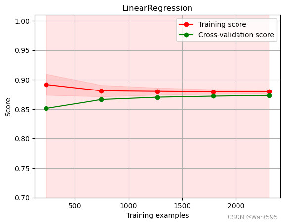
这段代码用于绘制学习曲线，可以通过观察学习曲线来判断模型是否存在欠拟合或过拟合问题。具体步骤如下：

1. 定义一个绘制学习曲线的函数plot_learning_curve，该函数的输入参数包括模型估计器estimator、标题title、输入变量X、输出变量y、纵轴取值范围ylim、交叉验证生成器cv、并行计算数n_jobs、训练集大小train_sizes。

2. 在函数内部，首先绘制了图像标题和横轴、纵轴标签。然后使用learning_curve函数生成学习曲线上的训练集数量(train_sizes)、训练集分数(train_scores)、测试集分数(test_scores)。

3. 通过计算平均分数和方差，绘制出训练集得分区间和测试集得分区间。

4. 绘制训练集得分和测试集得分的平均得分线。

5. 最后将图例放在最好的位置上，并返回绘制好的图像对象plt。

此处使用了shuffleSplit来进行交叉验证，shuffleSplit是一种将数据集随机化、划分成训练集和测试集的一种方法，它会随机地将数据分为N份，然后对于每一份N，N-1份作为训练集，剩下1份作为测试集，以此来生成交叉验证的训练集和测试集。然后利用所得到的训练集和测试集来得到训练集大小和训练得分、测试得分数据。

（2）验证曲线

import matplotlib.pyplot as plt
import numpy as np
from sklearn.linear_model import SGDRegressor
from sklearn.model_selection import validation_curve
X = train_data2[test_data2.columns].values
y = train_data2['target'].values
param_range = [0.1, 0.01, 0.001, 0.0001, 0.00001, 0.000001]
train_scores, test_scores = validation_curve(SGDRegressor(max_iter=1000, tol=1e-3, penalty='l1'), X, y, param_name="alpha", param_range=param_range, cv=10, scoring='r2', n_jobs=1)
train_scores_mean = np.mean(train_scores, axis=1)
train_scores_std = np.std(train_scores, axis=1)
test_scores_mean = np.mean(test_scores, axis=1)
test_scores_std = np.std(test_scores, axis=1)
plt.title("Validation Curve with SGDRegressor")
plt.xlabel("alpha")
plt.ylabel("Score")
plt.ylim(0.0, 1.1)
plt.semilogx(param_range, train_scores_mean, label="Training score", color='r')
plt.fill_between(param_range, train_scores_mean - train_scores_std,train_scores_mean + train_scores_std,alpha=0.2,color='r')
plt.semilogx(param_range, test_scores_mean, label='Cross-validation score', color='g')
plt.fill_between(param_range, test_scores_mean - test_scores_std,test_scores_mean + test_scores_std,alpha=0.2,color='g')
plt.legend(loc='best')
plt.show()

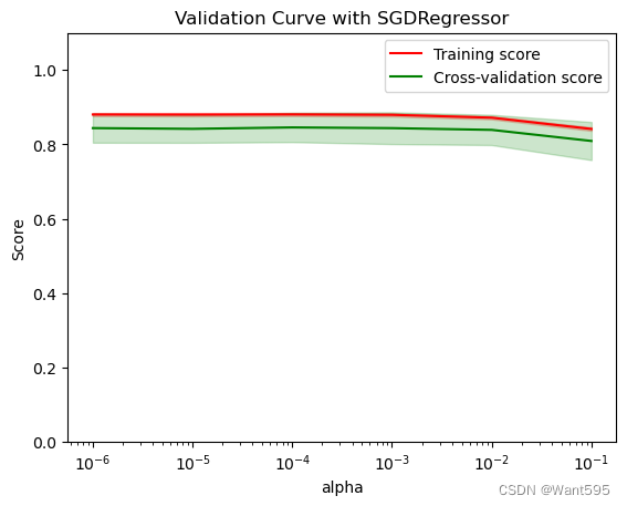
这段代码用于绘制验证曲线，可以通过观察验证曲线来选择模型的最优参数。具体步骤如下：

1. 通过validation_curve函数生成不同参数取值下的训练集得分和测试集得分。

2. 计算训练集得分和测试集得分的平均值和标准差。

3. 绘制图像标题和横轴、纵轴标签。

4. 绘制训练集得分和测试集得分的平均得分线。

5. 绘制训练集得分和测试集得分的得分区间。

6. 显示图例和图像。

此处使用了SGDRegressor来进行模型训练，使用了L1正则化来对模型进行约束，将模型中的权重限定在一个范围之内，以避免过拟合。通过变换参数alpha的值，我们可以得到不同参数取值下的训练集得分和测试集得分，并通过可视化来选择最优的alpha取值。

写在后面

我是一只有趣的兔子，感谢你的喜欢！

​

这篇关于机器学习实战：基于sklearn的工业蒸汽量预测的文章就介绍到这儿，希望我们推荐的文章对编程师们有所帮助！

---